En Machine Learning, we use various types of algorithms to allow machines to learn the relationships within the data provided and make predictions based on patterns or rules identified in the data set. Then, regression is a machine learning technique where the model predicts the output as a continuous numeric value.

Source: https://www.hindish.com
Regression analysis is often used in finance, investments and others, y descubre la relación entre una sola variableIn statistics and mathematics, a "variable" is a symbol that represents a value that can change or vary. There are different types of variables, and qualitative, that describe non-numerical characteristics, and quantitative, representing numerical quantities. Variables are fundamental in experiments and studies, since they allow the analysis of relationships and patterns between different elements, facilitating the understanding of complex phenomena.... dependent (target variable) which depends on several independent. For instance, predict house prices, the stock market or an employee's salary, etc. are the most common
regression problems.
The algorithms that we are going to cover are:
1. Linear regression
2. Decisions Tree
3. Support vector regression
4. Loop regression
5. Random forest
1. Linear regression
La regresión lineal es un algoritmo de aprendizaje automático que se utiliza para el supervised learningSupervised learning is a machine learning approach where a model is trained using a set of labeled data. Each input in the dataset is associated with a known output, allowing the model to learn to predict outcomes for new inputs. This method is widely used in applications such as image classification, speech recognition and trend prediction, highlighting its importance in.... Linear regression performs the task of predicting a dependent variable (objective) as a function of the given independent variables. Then, this regression technique finds a linear relationship between a dependent variable and the other independent variables given. Therefore, the name of this algorithm is Linear Regression.
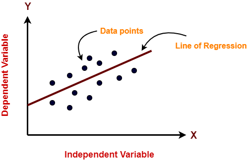
In the figure"Figure" is a term that is used in various contexts, From art to anatomy. In the artistic field, refers to the representation of human or animal forms in sculptures and paintings. In anatomy, designates the shape and structure of the body. What's more, in mathematics, "figure" it is related to geometric shapes. Its versatility makes it a fundamental concept in multiple disciplines.... anterior, on the X axis is the independent variable and on the Y axis is the output. The regression line is the line that best fits a model. And our main objective in this algorithm is to find the line that best fits.
Pros:
- Linear regression is easy to implement.
- Less complexity compared to other algorithms.
- Linear regression can cause overfitting, but it can be avoided by using some dimensionality reduction techniques, técnicas de regularizationRegularization is an administrative process that seeks to formalize the situation of people or entities that operate outside the legal framework. This procedure is essential to guarantee rights and duties, as well as to promote social and economic inclusion. In many countries, Regularization is applied in migratory contexts, labor and tax, allowing those who are in irregular situations to access benefits and protect themselves from possible sanctions.... y validación cruzada.
Cons:
- Outliers seriously affect this algorithm.
- It oversimplifies real-world problems by assuming a linear relationship between variables, therefore not recommended for practical use cases.
Implementation
import numpy as np
from sklearn.linear_model import LinearRegression
X = np.array([[2, 1], [3, 2], [4, 2], [5, 3]])
# y = 1 * x_0 + 2 * x_1 + 3
y = np.dot(X, np.array([1, 2])) + 3
lr = LinearRegression().fit(X, Y)
lr.predict(np.array([[1, 5]]))

Output
array([14.])
2. Decisions Tree
Decision tree models can be applied to all those data that contain numerical characteristics and categorical characteristics. Decision trees are good at capturing the non-linear interaction between the characteristics and the target variable.. Decision trees coincide in a way with human-level thinking, so it is very intuitive to understand the data.
Source: https://dinhanhthi.com
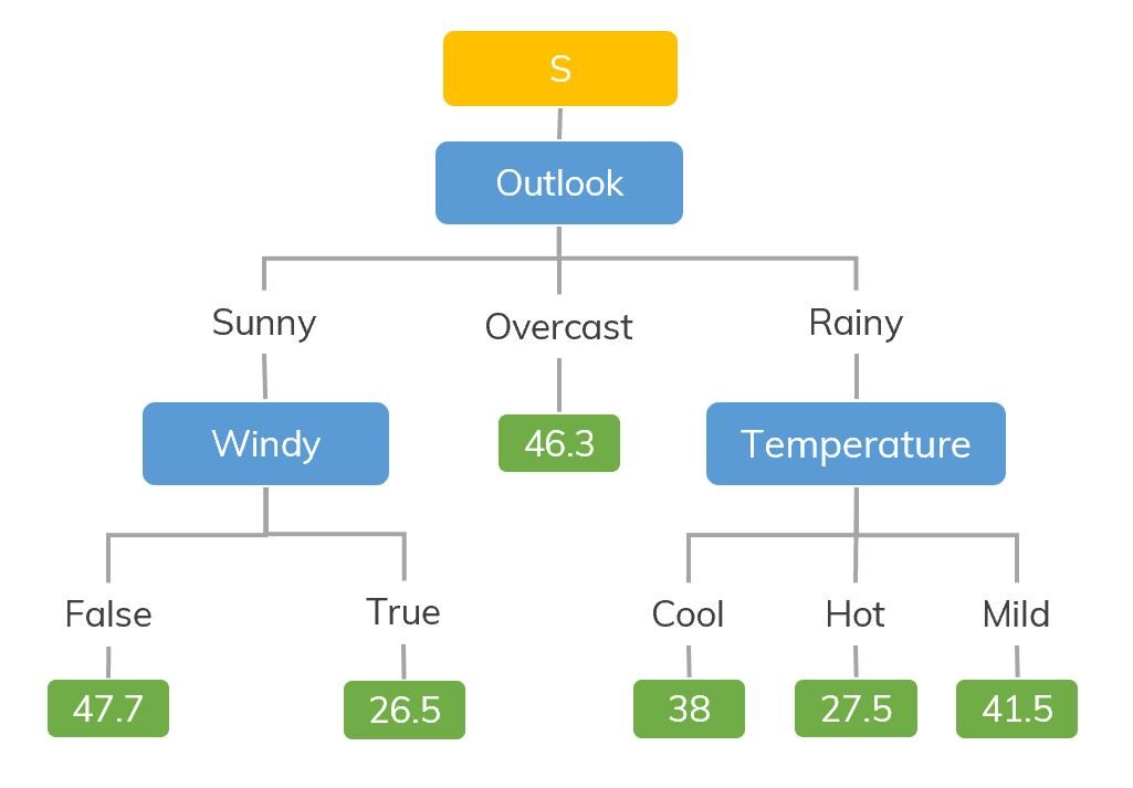
For instance, if we are classifying how many hours a child plays in a particular climate, the decision tree looks a bit like this in the picture.
Then, in summary, un árbol de decisiones es un árbol donde cada nodeNodo is a digital platform that facilitates the connection between professionals and companies in search of talent. Through an intuitive system, allows users to create profiles, share experiences and access job opportunities. Its focus on collaboration and networking makes Nodo a valuable tool for those who want to expand their professional network and find projects that align with their skills and goals.... representa una característica, each branch represents a decision and each leaf represents an outcome (numerical value for regression).
Pros:
- Easy to understand and interpret, visually intuitive.
- Can work with numerical and categorical characteristics.
- Requires little data pre-processing: no need for one-hot encoding, dummy variables, etc.
Cons:
- Tends to over-adjust.
- A small change in the data tends to make a big difference in the tree structure, what causes instability.
Implementation
import numpy as np
from sklearn.tree import DecisionTreeRegressor
rng = np.random.RandomState(1)
X = np.sort(5 * rng.rand(80, 1), axis=0)
y = np.sin(X).ravel()
Y[::5] += 3 * (0.5 - rng.rand(16))
# Fit regression model
regr = DecisionTreeRegressor(max_depth=2)
regr.fit(X, Y)
# Predict
X_test = np.arange(0.0, 5.0, 1)[:, e.g. newaxis]
result = regr.predict(X_test)
print(result)

Output:
[ 0.05236068  0.71382568  0.71382568  0.71382568 -0.86864256]
3. Support vector regression
You must have heard of SVM, namely, Support Vector Machine. SVR also uses the same idea of SVM but here it tries to predict the actual values. This algorithm uses hyperplanes to segregate the data. In case this separation is not possible, entonces usa el truco del kernel donde la dimension"Dimension" It is a term that is used in various disciplines, such as physics, Mathematics and philosophy. It refers to the extent to which an object or phenomenon can be analyzed or described. In physics, for instance, there is talk of spatial and temporal dimensions, while in mathematics it can refer to the number of coordinates necessary to represent a space. Understanding it is fundamental to the study and... aumenta y luego los puntos de datos se vuelven separables por un hiperplano.
Source: https://www.medium.com
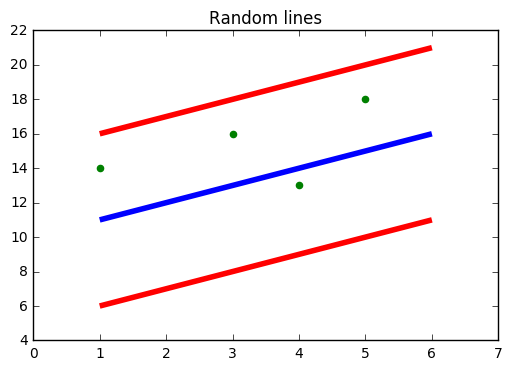
In the figure above, the blue line is the hyperplane; The red line is the limit line
All data points are within the boundary line (Red line). The main objective of SVR is basically to consider the points that are within the limit line.
Pros:
- Robust to outliers.
- Excellent generalizability
- High prediction accuracy.
Cons:
- Not suitable for large data sets.
- They don't work very well when the dataset has more noise.
Implementation
from sklearn.svm import SVR
import numpy as np
rng = np.random.RandomState(1)
X = np.sort(5 * rng.rand(80, 1), axis=0)
y = np.sin(X).ravel()
Y[::5] += 3 * (0.5 - rng.rand(16))
# Fit regression model
svr = SVR().fit(X, Y)
# Predict
X_test = np.arange(0.0, 5.0, 1)[:, e.g. newaxis]
svr.predict(X_test)
Output:
array([-0.07840308,  0.78077042,  0.81326895,  0.08638149, -0.6928019 ])
4. Loop regression
- LASSO stands for Absolute Minimum Selection Shrinkage Operator. La contracción se define básicamente como una restricción de atributos o parametersThe "parameters" are variables or criteria that are used to define, measure or evaluate a phenomenon or system. In various fields such as statistics, Computer Science and Scientific Research, Parameters are critical to establishing norms and standards that guide data analysis and interpretation. Their proper selection and handling are crucial to obtain accurate and relevant results in any study or project.....
- The algorithm works by finding and applying a constraint to the attributes of the model that cause the regression coefficients of some variables to reduce to zero..
- Variables with a regression coefficient of zero are excluded from the model.
- Therefore, loop regression analysis is basically a method of variable selection and contraction and helps to determine which of the predictors are most important.
Pros:
Cons:
- LASSO will select only one feature from a group of correlated features
- Selected features may be highly skewed.
Implementation
from sklearn import linear_model
import numpy as np
rng = np.random.RandomState(1)
X = np.sort(5 * rng.rand(80, 1), axis=0)
y = np.sin(X).ravel()
Y[::5] += 3 * (0.5 - rng.rand(16))
# Fit regression model
lassoReg = linear_model.Lasso(alpha=0.1)
lassoReg.fit(X,Y)
# Predict
X_test = np.arange(0.0, 5.0, 1)[:, e.g. newaxis]
lassoReg.predict(X_test)
Output:
array([ 0.78305084,  0.49957596,  0.21610108, -0.0673738 , -0.35084868])
5. Random Forest Regresser
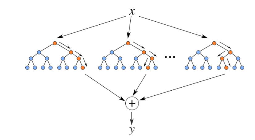
Random forests are a set (combination) decision trees. It is a supervised learning algorithm that is used for classification and regression. Input data is passed through multiple decision trees. Se ejecuta construyendo un número diferente de árboles de decisión en el momento del trainingTraining is a systematic process designed to improve skills, physical knowledge or abilities. It is applied in various areas, like sport, Education and professional development. An effective training program includes goal planning, regular practice and evaluation of progress. Adaptation to individual needs and motivation are key factors in achieving successful and sustainable results in any discipline.... y generando la clase que es el modo de las clases (for classification) or mean prediction (for regression) of individual trees.
Source: https://levelup.gitconnected.com
Pros:
- Good for learning complex and non-linear relationships
- Very easy to interpret and understand.
Cons:
- They are prone to over-adjusting
- Using larger random forest pools for higher performance slows down their speed and then they also require more memory.
Implementation
from sklearn.ensemble import RandomForestRegressor
from sklearn.datasets import make_regression
X, y = make_regression(n_features=4, n_informative=2, random_state=0, shuffle=False)
rfr = RandomForestRegressor(max_depth=3)
rfr.fit(X, Y)
print(rfr.predict([[0, 1, 0, 1]]))

Output:
[33.2470716]
Final notes
These are some popular regression algorithms, there are many more and also advanced algorithms. Explore them too. You can also follow these classification algorithms to increase your machine learning knowledge.
Thanks for reading if you got here 🙂
Let's connect LinkedIn
The media shown in this article is not the property of Analytics Vidhya and is used at the author's discretion.


