
This article was published as part of the Data Science Blogathon
According to experts, the 80% of the world's data is in the form of unstructured data (images, videos, text, etc.). This data could be generated by tweets / social media posts, call transcripts, survey or interview reviews, text messages on blogs, forums, news, etc.
It is humanly impossible to read all the text on the web and find patterns. But nevertheless, there is definitely a need for the company to analyze this data to take better actions.
One of those processes for obtaining knowledge from textual data is sentiment analysis. To obtain the data for sentiment analysis, one can directly scrape content from web pages using different web scraping techniques.
If you are new to web scraping, do not hesitate to consult my article “Web scraping with Python: BeautifulSoup”.
What is sentiment analysis?
Sentiment analysis (also known as opinion mining or emotion AI) is a subfield of NLP that measures the inclination of people's opinions (positive / negative / neutral) within unstructured text.
Sentiment analysis can be performed using two approaches: rule-based, machine learning based.
Few applications of sentiment analysis
- Market analysis
- Social media monitoring
- Analysis of customer feedback: analysis of brand opinion or reputation
- Market research
What is natural language processing (PNL)?
Natural language is the way we, the humans, we communicate with each other. It can be voice or text. NLP is the automatic manipulation of natural language by software. NLP is a higher level term and is the combination of Natural language understanding (NLU) Y Natural language generation (NLG).
PNL = NLU + NLG
Some of Python's natural language processing libraries (NLP) son:
- Natural Language Toolkit (NLTK)
- TextBlob
- SPACE
- Gensim
- CoreNLP
Hope we have a basic understanding of the terms Sentiment Analysis, PNL.
This article focuses on the rules-based approach to sentiment analysis..
Rules-based approach
This is a practical approach to analyze text without training or using machine learning models. The result of this approach is a set of rules based on which text is labeled positive. / negative / neutral. These rules are also known as lexicons. Therefore, the rule-based approach is called the lexical-based approach.
The widely used lexical-based approaches are TextBlob, VADER, SentiWordNet.
Data preprocessing steps:
- Cleaning up the text
- Tokenización
- Enrichment: point of sale labeling
- Noise word removal
- Get the root words
Before delving into the steps above, let me import the text data from a txt file.
Import a text file using Pandas read CSV function
# install and import pandas library
import pandas as pd
# Creating a pandas dataframe from reviews.txt file
data = pd.read_csv('reviews.txt', sep='t')
data.head()
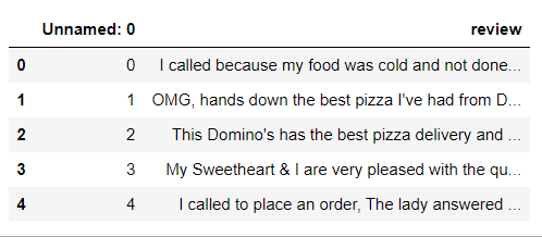
This doesn't look good. Then, now we will release the “Nameless: 0 ″ column using the df.drop function.
mydata = data.drop('Unnamed: 0', axis=1)
mydata.head()
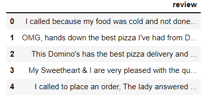
Our dataset has a total of 240 observations (reviews).
Paso 1: Clean up the text
In this step, we need to remove the special characters, text numbers. We can use the regular expression operations Python library.
# Define a function to clean the text
def clean(text):
# Removes all special characters and numericals leaving the alphabets
    text = re.sub('[^ A-Za-z]+', ' ', text)
    return text

# Cleaning the text in the review column
mydata['Cleaned Reviews'] = mydata['review'].apply(clean)
mydata.head()
Explanation: "Clean" is the function that takes text as input and returns it without punctuation or numbers. We apply it to the column ‘review’ and we create a new column ‘Clean reviews’ with clean text.
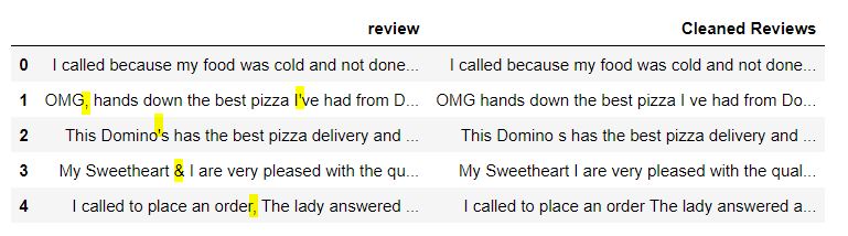
Genial, look at the picture above, all special characters and numbers are removed.
Paso 2: Tokenización
Tokenization is the process of dividing text into smaller pieces called Tokens. Can be done at the sentence level (sentence tokenization) or by word (word tokenization).
I will perform tokenization at the word level using tokenizar nltk word_tokenize function ().
Note: Since our text data is a bit big, I will illustrate the steps first 2-5 with little example sentences.
Say we have a prayer “This is an article on sentiment analysis.“. Can be divided into small pieces (records) as it's shown in the following.

Paso 3: Enrichment: POS labeling
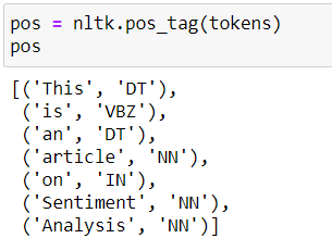
Labeling Parts of Speech (POS) is a process of converting each token into a tuple that has the form (word, label). POS tagging is essential to preserve the context of the word and is essential for stemming.
This can be achieved using nltk pos_tag function.
Below are the POS tags of the example sentence “This is an article on opinion analysis”.
See the list of possible pos de labels. here.
Paso 4: noise word removal
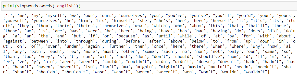
English stopwords are words that contain very little useful information. We need to remove them as part of the text preprocessing. nltk has a stopword list for each language.
See the stop words in English.
Example of stopword removal:

The empty words This, is, an, on are removed and the exit sentence is ‘Article opinion analysis’.
Paso 5: get the root words
A root is part of a word responsible for its lexical meaning. The Two Popular Techniques for Getting the Root Words / root are Stemming and Lemmatization.
The key difference is that Stemming often gives some nonsense root words, since it just cuts some characters at the end. Stemming provides meaningful roots, but nevertheless, requires POS tags of the words.
Example to illustrate the difference between Stemming and Lematization: Click here to get the code

If we look at the previous example, Stemming's output is Stem and Lemmatizatin's output is Lemma.
By the word look, the stem glanc Has no sense. Considering that, the motto look it is perfect.
Now we understood the steps 2-5 taking simple examples. Without forther delay, let's go back to our real problem.
Code for steps 2 a 4: tokenización, POS labeling, noise word removal
import nltk
nltk.download('punkt')
from nltk.tokenize import word_tokenize
from nltk import pos_tag
nltk.download('stopwords')
from nltk.corpus import stopwords
nltk.download('wordnet')
from nltk.corpus import wordnet

# POS tagger dictionary
pos_dict = {'J':wordnet.ADJ, 'V':wordnet.VERB, 'N':wordnet.NOUN, 'R':wordnet.ADV}
def token_stop_pos(text):
    tags = pos_tag(word_tokenize(text))
    newlist = []
    for word, tag in tags:
        if word.lower() not in set(stopwords.words('english')):
        newlist.append(tuple([word, pos_dict.get(tag[0])]))
    return newlist

mydata['POS tagged'] = mydata['Cleaned Reviews'].apply(token_stop_pos)
mydata.head()
Explanation: token_stop_pos is the function that takes the text and performs the tokenization, remove stopwords and tag the words in your POS. We apply it to the column ‘Clean reviews’ and we create a new column for the 'POS tagged' data.
As mentioned earlier, to get the precise motto, WordNetLemmatizer requires 'n' shaped POS tags, ‘a’, etc. But the POS tags obtained from pos_tag have the form 'NN', ‘ADJ’, etc.
To assign pos_tag to wordnet tags, we create a pos_dict dictionary. Any pos_tag that starts with J is mapped to wordnet.ADJ, any pos_tag that starts with R is mapped to wordnet.ADV, and so on.
Our interest tags are Noun, Adjective, Adverb, Verb. Anything from these four is assigned to None.
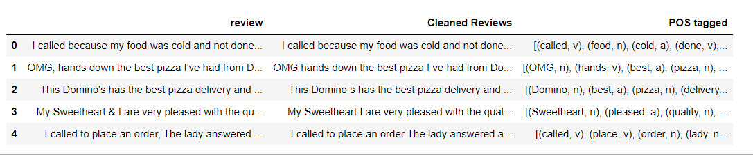
In the figure"Figure" is a term that is used in various contexts, From art to anatomy. In the artistic field, refers to the representation of human or animal forms in sculptures and paintings. In anatomy, designates the shape and structure of the body. What's more, in mathematics, "figure" it is related to geometric shapes. Its versatility makes it a fundamental concept in multiple disciplines.... anterior, we can see that each word in the column ‘POS labeled’ maps to your POS from pos_dict.
Code for step 5: get the root words – Lematización
from nltk.stem import WordNetLemmatizer
wordnet_lemmatizer = WordNetLemmatizer()
def lemmatize(pos_data):
    lemma_rew = " "
    for word, pos in pos_data:
    if not pos:
        lemma = word
        lemma_rew = lemma_rew + " " + lemma
    else:
        lemma = wordnet_lemmatizer.lemmatize(word, pos = pos)
        lemma_rew = lemma_rew + " " + lemma
    return lemma_rew

mydata['Lemma'] = mydata['POS tagged'].apply(lemmatize)
mydata.head()
Explanation: lemmatize is a function that takes pos_tag tuples and gives the Lemma for each word in pos_tag based on the pos of that word. We apply it to the column 'POS labeled’ and we create a column ‘Lema’ to store the output.
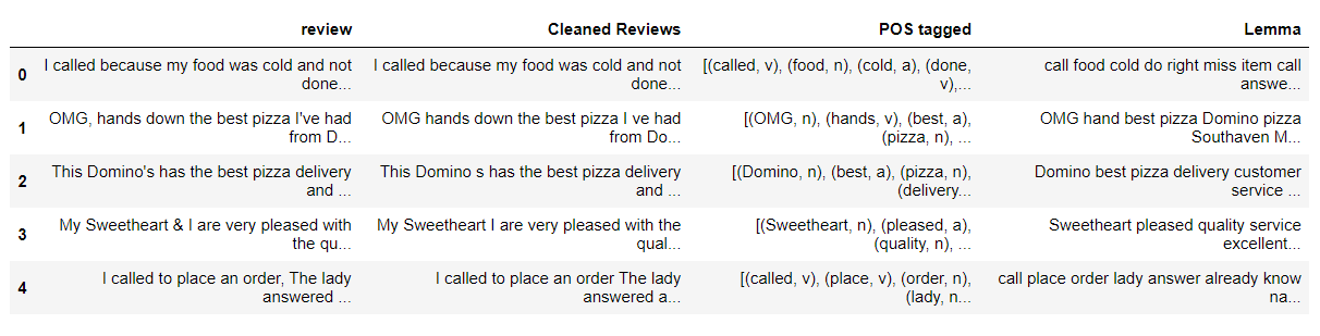
Yes, after a long trip, we are done with the pre-processing of the text.
Now, take a minute to look at the 'review' columns, 'Motto’ and watch how the text is processed.
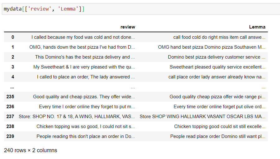
When we're done with data preprocessing, our final data looks clean. Take a short break and come back to continue the actual task.
Sentiment analysis using TextBlob:
TextBlob is a Python library for processing textual data. Provides a consistent API to dive into common natural language processing tasks (NLP), like tagging part of speech, noun phrase extraction, sentiment analysis and more.
The two measures used to analyze sentiment are:
- Polarity: talks about how positive or negative the opinion is.
- Subjectivity: talk about how subjective opinion is.
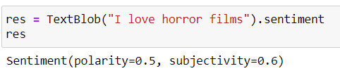
TextBlob (text) .sentiment gives us the Polarity values, Subjectivity.
Polarity varies from -1 a 1 (1 is more positive, 0 es neutral, -1 is more negative)
Subjectivity varies from 0 a 1 (0 it is very objective and 1 very subjective)
Python code:
from textblob import TextBlob
# function to calculate subjectivity
def getSubjectivity(review):
    return TextBlob(review).sentiment.subjectivity
    # function to calculate polarity
    def getPolarity(review):
        return TextBlob(review).sentiment.polarity

# function to analyze the reviews
def analysis(score):
    if score < 0:
        return 'Negative'
    elif score == 0:
        return 'Neutral'
    else:
        return 'Positive'
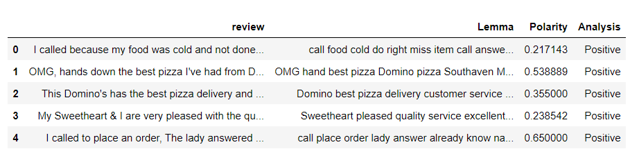
Explanation: functions created to obtain polarity values, subjectivity and label the review based on the polarity score.
Create a new data frame with the revision, Lemma columns and apply the above functions
fin_data = pd.DataFrame(mydata[['review', 'Lemma']])
# fin_data['Subjectivity'] = fin_data['Lemma'].apply(getSubjectivity)
fin_data['Polarity'] = fin_data['Lemma'].apply(getPolarity)
fin_data['Analysis'] = fin_data['Polarity'].apply(analysis)
fin_data.head()
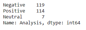
Count the number of positive reviews, negative and neutral.
tb_counts = fin_data.Analysis.value_counts()

tb_counts
Sentiment analysis with VADER
VADER stands for Valence Aware Dictionary and Sentiment Reasoner. Vader's sentiment doesn't just tell if the statement is positive or negative along with the intensity of the emotion.

The sum of the intensities pos, neg, new there 1. The compound varies from -1 a 1 y is the metric used to draw the overall sentiment.
positive if compound> = 0.5
neutral yes -0,5 <compound <0,5
negative yes -0,5> = compound
Python code:
from VaderSentiment.vaderSentiment import SentimentIntensityAnalyzer
analyzer = SentimentIntensityAnalyzer()
# function to calculate father sentiment
def father sentiment analysis(review):
    vs = analyzer.polarity_scores(review)
    return vs['compound']
    fin_data['Vader Sentiment'] = fin_data['Lemma'].apply(father sentiment analysis)
# function to analyse
def vader_analysis(compound):
    if compound >= 0.5:
        return 'Positive'
    elif compound <= -0.5 :
        return 'Negative'
    else:
        return 'Neutral'
fin_data['Vader Analysis'] = fin_data['Vader Sentiment'].apply(vader_analysis)
fin_data.head()
Explanation: Features built to get Vader scores and tag reviews based on composite scores
Count the number of positive reviews, negative and neutral.
father_counts = fin_data['Vader Analysis'].value_counts()
vader_counts
Sentiment analysis using SentiWordNet
SentiWordNet uses the databaseA database is an organized set of information that allows you to store, Manage and retrieve data efficiently. Used in various applications, from enterprise systems to online platforms, Databases can be relational or non-relational. Proper design is critical to optimizing performance and ensuring information integrity, thus facilitating informed decision-making in different contexts.... WordNet. It is important to get the POS, motto of each word. Then we will use the motto, POS to get the synonym sets (synsets). Then, we obtain the objective scores, negative and positive for all possible synthesizers or the first synthesizer and we label the text.
yes positive score> negative score, the feeling is positive
yes positive score <negative score, the feeling is negative
if positive score = negative score, the feeling is neutral
Python code:
nltk.download('sentiwordnet')
from nltk.corpus import sentiwordnet as swn
def sentiwordnetanalysis(pos_data):
    sentiment = 0
    tokens_count = 0
    for word, pos in pos_data:
        if not pos:
            continue
            lemma = wordnet_lemmatizer.lemmatize(word, pos = pos)
        if not lemma:
            continue
            synsets = wordnet.synsets(lemma, pos = pos)
        if not synsets:
            continue
            # Take the first sense, the most common
            synset = synsets[0]
            noise_synset = noise.senti_synset(synset.name())
            sentiment += swn_synset.pos_score() - swn_synset.neg_score()
            tokens_count += 1
            # print(swn_synset.pos_score(),swn_synset.neg_score(),swn_synset.obj_score())
        if not tokens_count:
            return 0
        if sentiment>0:
            return "Positive"
        if sentiment==0:
            return "Neutral"
        else:
            return "Negative"

fin_data['SWN analysis'] = mydata['POS tagged'].apply(sentiwordnetanalysis)
fin_data.head()
Explanation: We create a function to get the positive and negative scores for the first word of the synset and then label the text by calculating the sentiment as the difference of positive and negative scores.
Count the number of positive reviews, negative and neutral.
swn_counts= fin_data['SWN analysis'].value_counts()
swn_counts
Up to this point, We have seen the implementation of sentiment analysis using some of the popular lexicon-based techniques. Now quickly make a visualization and compare the results.
Visual representation of TextBlob results, VADER, SentiWordNet
We will chart the positive review count, negative and neutral for the three techniques.
import matplotlib.pyplot as plt
%matplotlib inline
plt.figure(figsize=(15,7))
plt.subplot(1,3,1)
plt.title("TextBlob results")
plt.pie(tb_counts.values, labels = tb_counts.index, explode = (0, 0, 0.25), autopct="%1.1f%%", shadow=False)
plt.subplot(1,3,2)
plt.title("VADER results")
plt.pie(vader_counts.values, labels = vader_counts.index, explode = (0, 0, 0.25), autopct="%1.1f%%", shadow=False)
plt.subplot(1,3,3)
plt.title("SentiWordNet results")
plt.pie(swn_counts.values, labels = swn_counts.index, explode = (0, 0, 0.25), autopct="%1.1f%%", shadow=False)
If we look at the image above, TextBlob and SentiWordNet results look a bit close, while the VADER results show a large variation.
Final notes:
Congratulations 🎉 to us. At the end of this article, We have learned the various steps of data preprocessing and the different lexical-based approaches to sentiment analysis. We compare the results of TextBlob, VADER, SentiWordNet using pie charts.
References:
See the full Jupyter notebook here hosted on GitHub.
The media shown in this article is not the property of Analytics Vidhya and is used at the author's discretion.





