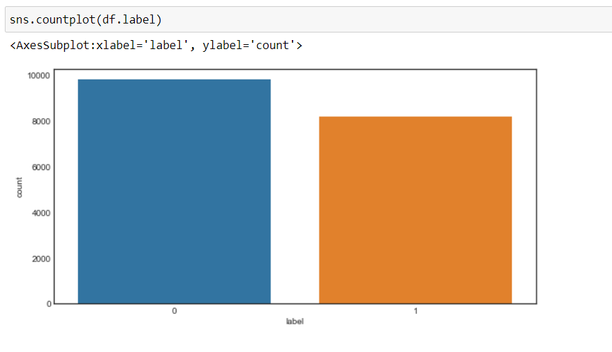
Now, we can see that our goal has changed to 0 Y 1, namely, 0 for negative and 1 for positive, and the data is more or less in a balanced state.
Data preprocessing
Now, we will pre-process the data before converting it to vectors and passing it to the machine learning model.
We will create a function for data preprocessing.
1. First, we will iterate through each record and use a regular phrase, we will remove any character apart from the alphabets.
2. Later, we will convert the string to lower case What, the word “Well” is different from the word “good”.
Why, not converted to lowercase, will cause a problem when we create vectors of these words, since two different vectors will be created for the same word that we do not want.
3. Later, we will look for stop words in the data and remove them. For words are commonly used words in a sentence like “the”, “a”, “a”, etc. that don't add much value.
4. Later, we will perform lematización in every word, namely, change the different forms of a word into a single element called a slogan.
A motto is a basic form of a word. For instance, “run”, “to run” Y “run” they are all forms of the same lexeme, where “run” is the motto. Therefore, we are converting all occurrences of the same lexeme to their respective motto.
5. And then return a corpus of processed data.
But first we will create a WordNetLemmatizer object and then we will do the transformation.
#object of WordNetLemmatizer
lm = WordNetLemmatizer()
def text_transformation(df_col):
    corpus = []
    for item in df_col:
        new_item = re.sub('[^ a-zA-Z]',' ',str(item))
        new_item = new_item.lower()
        new_item = new_item.split()
        new_item = [lm.lemmatize(word) for word in new_item if word not in set(stopwords.words('english'))]
        corpus.append(' '.join(str(x) for x in new_item))
    return corpus
corpus = text_transformation(df['text'])
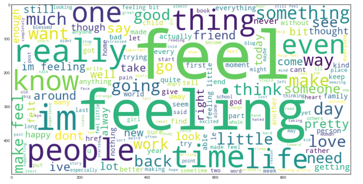
Now we will create a Word cloud. It is a data visualization technique used to represent text in such a way that the most frequent words appear enlarged compared to the less frequent words. This gives us a little idea of how the data looks after being processed through all the steps so far.
rcParams['figure.figsize'] = 20,8
word_cloud = ""
for row in corpus:
    for word in row:
        word_cloud+=" ".join(word)
wordcloud = WordCloud(width = 1000, height = 500,background_color="white",min_font_size = 10).generate(word_cloud)
plt.imshow(wordcloud)
Production:
Bag of words
Now, we will use the Bag of Words Model (BOW), used to represent text in the form of a bag of words, namely, grammar and word order in a sentence is not given any importance, However, the multiplicity , namely (the number of times a word appears in a document) is the main cause for concern.
Basically, describes the total occurrence of words within a document.
Scikit-Learn provides a neat way to perform the bag of words technique using CountVectorizer.
Now, we will convert the text data into vectors, adjusting and transforming the corpus we have created.
cv = CountVectorizer(ngram_range=(1,2))
traindata = cv.fit_transform(corpus)
X = traindata
y = df.label
We will take it ngram_range What (1,2) what does a bigrama mean.
Ngram is a sequence of 'n’ words in a row or sentence. ‘ngram_range’ is a parameter, that we use to give importance to the combination of words, What “social media” has a different meaning than “social” Y “media” separately.
We can experiment with the value of ngram_range parameter and select the option that gives the best results.
Now comes the machine learning model creation part and in this project, I am going to wear Random forest classifier, and we will adjust the hyperparameters using GridSearchCV.
GridSearchCV() will take the following parameters,
1. Estimator the model – RandomForestClassifier in our case
2. parameters: dictionary of hyperparameter names and their values
3. cv: means cross validation folds
4. return_train_score: returns the training scores of the different models
5. n_jobs – no. jobs to run in parallel (“-1” means all CPU cores will be used, which drastically reduces training time)
First, we will create a dictionary, “parameters” which will contain the values of different hyperparameters.
We will pass this as a parameter to GridSearchCV to train our random forest classifier model using all possible combinations of these parameters to find the best model.
parameters = {'max_features': ('auto','sqrt'),
             'n_estimators': [500, 1000, 1500],
             'max_depth': [5, 10, None],
             'min_samples_split': [5, 10, 15],
             'min_samples_leaf': [1, 2, 5, 10],
             'bootstrap': [True, False]}
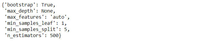
Now, we will adjust the data in the grid search and see the best parameter using the attribute “best_params_” by GridSearchCV.
grid_search = GridSearchCV(RandomForestClassifier(),parameters,cv=5,return_train_score=True,n_jobs=-1)
grid_search.fit(X,Y)
grid_search.best_params_
Production:
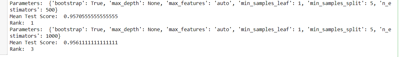
And later, we can see all the models and their respective parameters, the average test score and ranking, since GridSearchCV stores all results in the cv_results_ attribute.
for i in range(432):
    print('Parameters: ',grid_search.cv_results_['params'][i])
    print('Mean Test Score: ',grid_search.cv_results_['mean_test_score'][i])
    print('Rank: ',grid_search.cv_results_['rank_test_score'][i])
Departure: (a sample of the output)
Now, we will choose the best parameters obtained from GridSearchCV and create a final random forest classifier model and then train our new model.
rfc = RandomForestClassifier(max_features=grid_search.best_params_['max_features'],
                                      max_depth=grid_search.best_params_['max_depth'],
                                      n_estimators=grid_search.best_params_['n_estimators'],
                                      min_samples_split=grid_search.best_params_['min_samples_split'],
                                      min_samples_leaf=grid_search.best_params_['min_samples_leaf'],
                                      bootstrap=grid_search.best_params_['bootstrap'])
rfc.fit(X,Y)
Test data transformation
Now, we will read the test data and perform the same transformations that we did on the training data and finally evaluate the model on its predictions.
test_df = pd.read_csv('test.txt',delimiter=";",names=['text','label'])
X_test,y_test = test_df.text,test_df.label
#encode the labels into two classes , 0 and 1
test_df = custom_encoder(y_test)
#pre-processing of text
test_corpus = text_transformation(X_test)
#convert text data into vectors
testdata = cv.transform(test_corpus)
#predict the target
predictions = rfc.predict(testdata)
Model evaluation
We will evaluate our model using various metrics such as Accuracy Score, Precision Score, Recall Score, Confusion Matrix and we will create a roc curve to visualize how our model performed.
rcParams['figure.figsize'] = 10,5
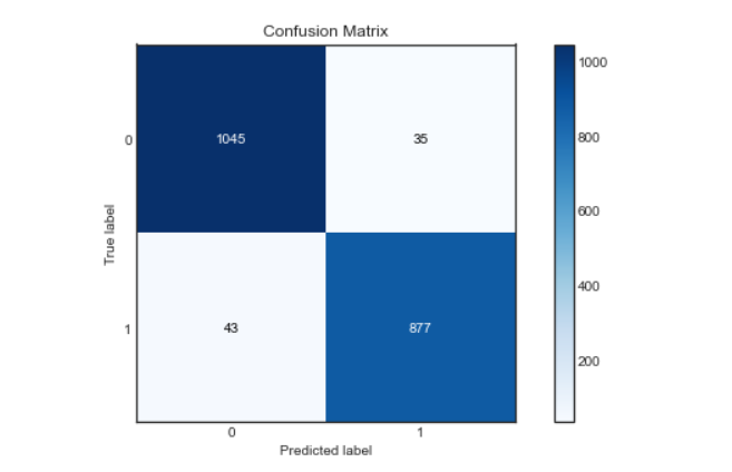
plot_confusion_matrix(y_test,predictions)
acc_score = accuracy_score(y_test,predictions)
pre_score = precision_score(y_test,predictions)
rec_score = recall_score(y_test,predictions)
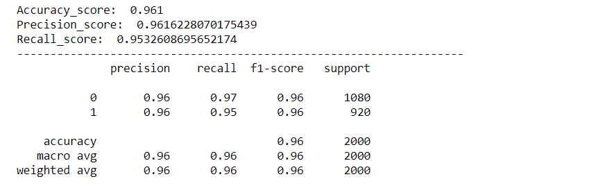
print('Accuracy_score: ',acc_score)
print('Precision_score: ',pre_score)
print('Recall_score: ',rec_score)
print("-"*50)
cr = classification_report(y_test,predictions)
print(cr)
Production:
Confusion matrix:
Roc curve:
We will find the probability of the class using the predict_proba method () of Random Forest Classifier and then we will plot the curve roc.
predictions_probability = rfc.predict_proba(testdata)
fpr,tpr,thresholds = roc_curve(y_test,predictions_probability[:,1])
plt.plot(fpr,tpr)
plt.plot([0,1])
plt.title('ROC Curve')
plt.xlabel('False Positive Rate')
plt.ylabel('True Positive Rate')
plt.show()
As we can see, our model worked very well in classifying feelings, with a precision score, accuracy and recovery of approx. 96%. And the roc curve and confusion matrix are also excellent, which means that our model can classify the labels accurately, with less chance of error.
Now, we will also check the custom input and let our model identify the sentiment of the input statement.
Predict for custom input:
def expression_check(prediction_input):
    if prediction_input == 0:
        print("Input statement has Negative Sentiment.")
    elif prediction_input == 1:
        print("Input statement has Positive Sentiment.")
    else:
        print("Invalid Statement.")
# function to take the input statement and perform the same transformations we did earlier
def sentiment_predictor(input):
    input = text_transformation(input)
    transformed_input = cv.transform(input)
    prediction = rfc.predict(transformed_input)
    expression_check(prediction)
input1 = ["Sometimes I just want to punch someone in the face."]
input2 = ["I bought a new phone and it's so good."]
sentiment_predictor(input1)
sentiment_predictor(input2)
Production:

Hurray, since we can see that our model accurately classified the feelings behind the two sentences.
If you like this article, follow me in LinkedIn.
And you can get the complete code and output from here.
Output images are kept here for reference.
The end?
The media shown in this article is not the property of Analytics Vidhya and is used at the author's discretion.


