This article was published as part of the Data Science Blogathon
Introduction
The ultimate goal of this blog is to predict the sentiment of a given text using python, where we use NLTK, also known as Natural Language Processing Toolkit, a Python package specially created for text-based analysis. Then, with a few lines of code, we can easily predict whether a sentence or a review (used in the blog) is it a positive or negative review.

Before moving directly to implementation, allow me briefly the steps involved to get an idea of the analytics approach. These are namely:
1. Import of required modules
2. Dataset import
3. Data preprocessing and visualization
4. Model building
5. Prediction
So let's focus on each step in detail.
1. Import of required modules:
Then, as we all know, it is necessary to import all the modules that we are going to use initially. So let's do it as the first step of our practice.
import numpy as np                  #linear algebra
import pandas as pd                 # data processing, CSV file I / O (e.g. pd.read_csv)
import matplotlib.pyplot as plt     #For Visualisation
%matplotlib inline
import seaborn as sns               #For better Visualisation
from bs4 import BeautifulSoup       #For Text Parsing
Here we are importing all the necessary basic import modules, namely, numpy, pandas, matplotlib, seaborn y beautiful soup, each with its own use case. Although we will use some other modules, excluding them, we will understand them while we use them.
2. Dataset import:
In fact, I had downloaded the Kaggle dataset quite some time ago, so I don't have the link to the dataset. Then, to get the dataset and code, I will put the link of the Github repository so that everyone has access to it. Now, to import the dataset, we have to use the pandas ‘read_csv method’ followed by the file path.
data = pd.read_csv('Reviews.csv')
If we print the data set, we could see that there are ‘568454 rows × 10 columns', which is quite big.
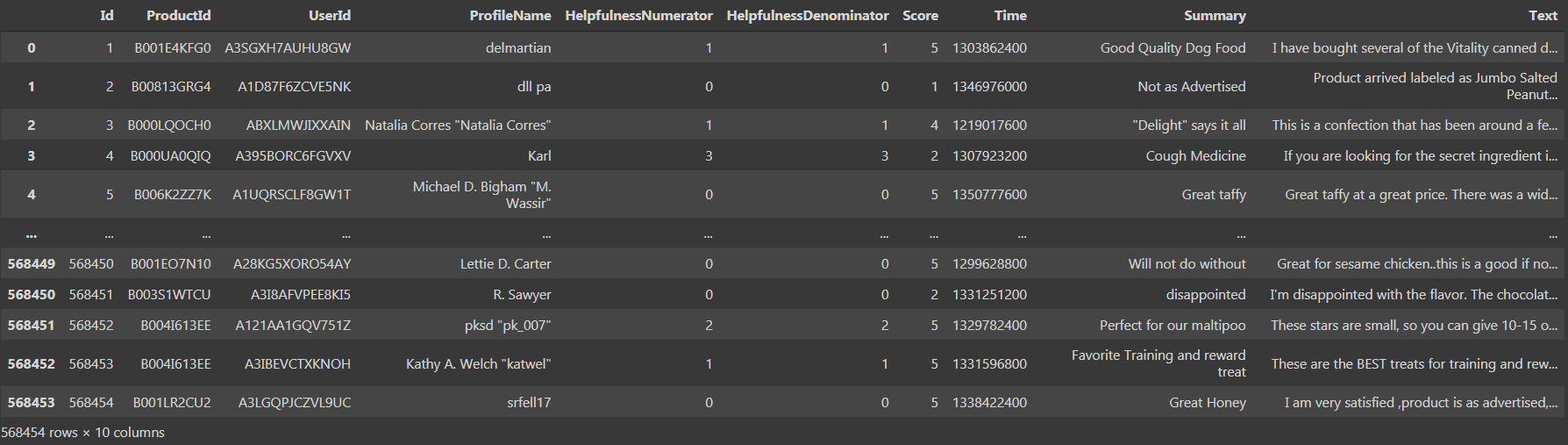
We see that there is 10 columns, namely, ‘Id’, ‘Utility numerator’, ‘Utility denominator’, 'Score’ and ‘Time’ as data type int64 and 'ProductId', ‘UserId’, ‘ProfileName’, 'Summary', 'Text’ as object data type. Now let's move on to the third step, namely, data preprocessing and visualization.
3. Data preprocessing and visualization:
Now we have access to the data and then we clean it. Using the 'isnull method (). Sum ()’ we could easily find the total number of missing values in the data set.
data.isnull().sum()
If we run the above code as a cell, we found that there is 16 Y 27 null values in 'ProfileName columns’ y ‘Summary’ respectively. Now, we have to replace the null values with the central tendency or remove the respective rows containing the null values. With such a large number of rows, removing solo 43 rows containing the null values would not affect the overall precision of the model. Therefore, it is advisable to eliminate 43 rows using the 'dropna' method.
data = data.dropna()
Now, I have updated the old dataframe instead of creating a new variable and storing the new dataframe with the clean values. Now, again, when we check the data frame, we found that there is 568411 rows and the same 10 columns, which means that 43 rows that had the null values have been removed and now our dataset is cleaned. Continuing, we have to preprocess the data in such a way that the model can use it directly.
Para preprocessor, we use the column ‘Score’ in the data frame to have scores ranging from '1’ a ‘5’, where '1’ means a negative review and '5’ means a positive review. But it is better to have the score initially in a range of ‘0’ a ‘2’ where ‘0’ means a negative review, ‘1’ means a neutral review and '2’ means a positive review. It is similar to coding in Python, but here we don't use any built-in functions, but we explicitly run a for where loop and create a new list and add the values to the list.
a=[]
for i in data['Score']:
    if i <3:
        a.append(0)
    if i==3:
        a.append(1)
    if i>3:
        a.append(2)
Assuming that the 'Score’ is in the range of ‘0’ a ‘2’, We consider them negative reviews and add them to the list with a score of ‘0’, what does negative review mean. Now, if we graph the values of the scores present in the list 'a’ as the nomenclature used above, we found that there is 82007 negative reviews, 42638 neutral reviews and 443766 positive reviews. We can clearly find that approximately the 85% of the reviews in the dataset have positive reviews and the remainder are negative or neutral reviews. This could be more clearly visualized and understood with the help of a counting plot in the seaborn library.
sns.countplot(a)
plt.xlabel('Reviews', color="red")
plt.ylabel('Count', color="red")
plt.xticks([0,1,2],['Negative','Neutral','Positive'])
plt.title('COUNT PLOT', color="r")
plt.show()
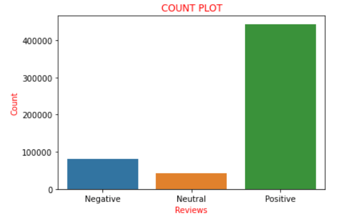
Therefore, the above plot clearly portrays all the sentences described above pictorially. Now I convert the list 'to’ that we had previously coded in a new column called 'feeling’ to data frame, namely, 'data'. Now comes a twist in which we create a new variable, let's say ‘final_dataset’ where I consider only the column ‘Feeling’ and ‘text’ of the data frame, which is the new data frame we are going to work on for the next part. The reason behind this is that all the remaining columns are considered those that do not contribute to the sentiment analysis., Thus, without discarding them, we consider the data frame to exclude those columns. Therefore, that is the reason to choose only the columns ‘Text’ and 'Feeling'. We code the same as below:
data['sentiment']=a
final_dataset = data[['Text','sentiment']]
final_dataset
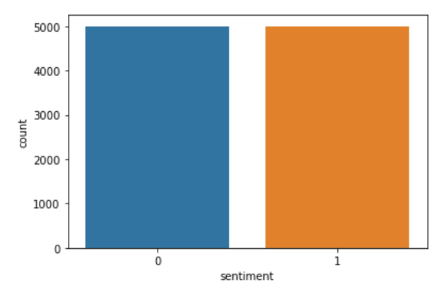
Now, if we print the ‘final_dataset’ and we find the way, we got to know that there is 568411 rows and only 2 columns. From the final_dataset, If we find out that the number of positive feedback is 443766 entries and the number of negative comments is 82007. Therefore, there is a big difference between positive and negative feedback. Therefore, there is more chance that the data will fit too much if we try to build the model directly. Therefore, we have to choose only a few inputs from the final_datset to avoid overfitting. Then, from various trials, I have found that the optimal value for the number of revisions to consider is 5000. Therefore, I create two new variables' datap’ and ‘date’ and randomly store 5000 positive and negative reviews on the variables respectively. The code that implements the same is below:
datap = data_p.iloc[np.random.randint(1,443766,5000), :]
datan = data_n.iloc[np.random.randint(1, 82007,5000), :]
len(data), len(datap)
Now I create a new variable called data and concatenate the values in 'datap’ and ‘date’.
data = pd.concat([datap,data])
len(data)
Now I create a new list called 'c’ and what I do is similar to the encoding but explicitly. I keep the negative reviews “0” What “0” and the positive reviews “2” before how “1” in “c”. Later, again I replace the sentiment values stored in 'c’ in column data. Later, to see if the code has been executed correctly, I draw the column ‘feeling’. The code that implements the same is:
c=[]
for i in data['sentiment']:
    if i==0:
        c.append(0)
    if i==2:
        c.append(1)
data['sentiment']=c
sns.countplot(data['sentiment'])
plt.show()
If we see the data, we can find that there are some HTML tags, as the data was originally sourced from actual ecommerce sites. Therefore, we can find that there are tags present that need to be removed, since they are not necessary for sentiment analysis. Therefore, we use the BeautifulSoup function that uses the 'html.parser’ and we can easily remove unwanted tags from reviews. To perform the task, I create a new column called 'review’ which stores the parsed text and drops the column called 'feeling’ to avoid redundancy. I have done the above task using a function called 'strip_html'. The code to do the same is the following:
def strip_html(text):
    soup = BeautifulSoup(text, "html.parser")
    return soup.get_text()
data['review'] = data['Text'].apply(strip_html)
data=data.drop('Text',axis=1)
data.head()
We have now come to the end of a tedious data visualization and preprocessing process. Therefore, now we can continue to the next step, namely, model building.
4. Construction model:
Before we jump directly to build the model we need, to do a little homework. We know that for humans to classify sentiment we need articles, determinants, conjunctions, punctuation marks, etc, as we can clearly understand and then rate the review. But this is not the case with machines, so they don't really need them to classify the feeling, but they are literally confused if they are present. Then, to perform this task like any other sentiment analysis, we need to use the 'nltk' library. NLTK son las siglas de ‘Natural Language Processing Toolkit’. This is one of the top libraries for doing sentiment analysis or any text-based machine learning project. Then, with the help of this library, i will first remove the punctuation marks and then remove the words that don't add a sentiment to the text. First I use a function called 'punc_clean’ which removes punctuation marks from each review. The code to implement the same is the following:
import nltk
def punc_clean(text):
    import string as st
    a=[w for w in text if w not in st.punctuation]
    return ''.join(a)
data['review'] = data['review'].apply(punc_clean)
data.head(2)
Therefore, the above code removes punctuation marks. Now, then, we have to remove the words that don't add a feeling to the sentence. These words are called “empty words”. List of almost all stopwords could be found here. Then, if we check the list of empty words, we can find that it also contains the word “no”. Therefore, it is necessary that we do not eliminate the “no” from “revision”, as it adds some value to the sentiment because it contributes to the negative sentiment. Therefore, we have to write the code in such a way that we remove other words except the “no”. The code to implement the same is:
def remove_stopword(text):
    stopword=nltk.corpus.stopwords.words('english')
    stopword.remove('not')
    a=[w for w in nltk.word_tokenize(text) if w not in stopword]
    return ' '.join(a)
data['review'] = data['review'].apply(remove_stopword)
Therefore, now we only have one step behind model building. The next reason is to assign each word in each review with a sentiment score. Then, to implement it, we need to use another library from the ‘sklearn module’ what is the 'TfidVectorizer’ which is present within ‘feature_extraction.text’. It is strongly recommended to go through the 'TfidVectorizer’ docs to get a clear understanding of the library. Has many parameters as input, coding, min_df, max_df, ngram_range, binary, dtype, use_idf and many more parameters, each with its own use case. Therefore, it is recommended to go through this Blog to get a clear understanding of how 'TfidVectorizer' works. The code that implements the same is:
from sklearn.feature_extraction.text import TfidfVectorizer
vectr = TfidfVectorizer(ngram_range=(1,2),min_df=1)
vectr.fit(data['review'])
vect_X = vectr.transform(data['review'])
Now is the time to build the model. Since it is a binary class classification sentiment analysis, namely, ‘1’ refers to a positive review and ‘0’ refers to a negative review. Then, it is clear that we need to use any of the classification algorithms. The one used here is the logistic regression. Therefore, we need to import 'LogisticRegression’ to use it as our model. Later, we need to fit all data as such because I felt it is good to test the data from brand new data instead of the available dataset. So I have adjusted the whole dataset. Then I use the '.score function ()’ to predict the model score. The code that implements the above mentioned tasks is as follows:
from sklearn.linear_model import LogisticRegression
model = LogisticRegression()
clf=model.fit(vect_X,data['sentiment'])
clf.score(vect_X,data['sentiment'])*100
If we run the above code snippet and check the model score, we get between 96 Y 97%, since the dataset changes every time we run the code, since we consider the data randomly. Therefore, we have successfully built our model which also with a good score. Then, Why wait to test how our model works in the real world scenario? So now we move on to the last and final step of the 'Prediction’ to test the performance of our model.
5. Prediction:
Then, to clarify the performance of the model, I have used two simple sentences "I love ice cream" and "I hate ice cream" that clearly refer to positive and negative feelings.. The result is as follows:
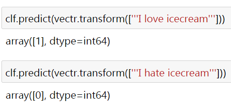
Here the '1’ and the ‘0’ refer to positive and negative sentiment respectively. Why aren't some real world reviews tested?? I ask you as readers to verify and prove the same. Most of the time you would get the desired output, but if that doesn't work, I ask you to try to change the parameters of the 'TfidVectorizer’ and set the model to 'LogisticRegression’ to get the required output. Then, for which I have attached the link to the code and the dataset here.
You connect with me through linkedin. Hope this blog is helpful in understanding how sentiment analysis is done practically with the help of Python codes. Thank you for seeing the blog.
The media shown in this article is not the property of DataPeaker and is used at the author's discretion.


