
This article was published as part of the Data Science Blogathon.
Introduction
is used to predict future values based on previously observed values and one of the best tools for trend analysis and future prediction.
What is time series data?
It is recorded at regular time intervals and the order of these data points is important. Therefore, any predictive model based on time series data will have time as variableIn statistics and mathematics, a "variable" is a symbol that represents a value that can change or vary. There are different types of variables, and qualitative, that describe non-numerical characteristics, and quantitative, representing numerical quantities. Variables are fundamental in experiments and studies, since they allow the analysis of relationships and patterns between different elements, facilitating the understanding of complex phenomena.... Independent. The output of a model would be the predicted value or rank at a specific time.
Time series analysis vs time series forecast
Let's talk about some possible confusion about time series analysis and forecasting. Time series forecasting is an example of predictive modeling, while time series analysis is a form of descriptive modeling.
For a new investor, the general research associated with the stock market or the stock market is not enough to make the decision. The common trend towards the stock market among society is highly risky for investment, so most people cannot make decisions based on common trends. seasonal variation and the constant flow of any indexThe "Index" It is a fundamental tool in books and documents, which allows you to quickly locate the desired information. Generally, it is presented at the beginning of a work and organizes the contents in a hierarchical manner, including chapters and sections. Its correct preparation facilitates navigation and improves the understanding of the material, making it an essential resource for both students and professionals in various areas.... will help new and existing investors understand and make the decision to invest in the stock market.
To solve these kinds of problems, time series forecasting is the best technique.
Stock Exchange
Stock markets are the places where individual and institutional investors come together to buy and sell stocks in a public place.. Today, these exchanges exist as electronic marketplaces.
That supply and demand help determine the price of each security or the levels at which participants in the stock market (investors and traders) are willing to buy or sell.
The concept behind how the stock market works is quite simple.. Operating much like an auction house, the stock market allows buyers and sellers to negotiate prices and carry out transactions.
Definition of ‘stock’
An action or action (also known as “capital” of a company) is a financial instrument that represents the ownership of a company
Machine learning in the stock market
The stock market is very unpredictable, any geopolitical change can affect the trend of stocks in the stock market, we have recently seen how covid-19 has impacted stock prices, so in financial data it is very difficult to do a reliable trend analysis. . the most efficient way to solve this type of problem is with the help of machine learning and the deep learningDeep learning, A subdiscipline of artificial intelligence, relies on artificial neural networks to analyze and process large volumes of data. This technique allows machines to learn patterns and perform complex tasks, such as speech recognition and computer vision. Its ability to continuously improve as more data is provided to it makes it a key tool in various industries, from health....
In this tutorial, we will solve this problem with the ARIMA model.
To know the seasonality, check my previous blog. And to get a basic understanding of ARIMA, I would recommend that you read this blog, this will help you better understand how time series analysis works.
Implement the stock price forecast
I will use nsepy library to extract historical data from SBIN.
Imports
import os
import warnings
warnings.filterwarnings(ignore)
from pylab import rcParams
rcParams['figure.figsize'] = 10, 6
from statsmodels.tsa.stattools import adfuller
from statsmodels.tsa.seasonal import seasonal_decompose
from statsmodels.tsa.arima_model import ARIMA
from pmdarima.arima import auto_arima
from sklearn.metrics import mean_squared_error, mean_absolute_error
import math
import numpy as np
from nsepy import get_history
from datetime import date
import matplotlib.pyplot as plt
import seaborn as sns
import pandas as pd
Run the below code to extract the historical data:
sbin = get_history(symbol="SBIN",
                   start=date(2000,1,1),
                   end=date(2020,11,1))
sbin.head()
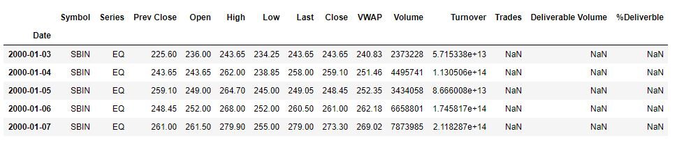
The data shows the stock price of SBIN from 2020-1-1 to 2020-11-1. The goal is to create a model that will forecast
the closing price of the stock.
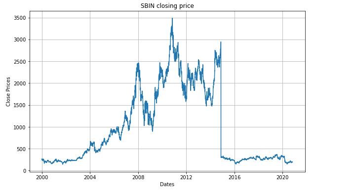
Let's create a visualization that will show the daily closing price of the stock.
plt.figure(figsize=(10,6))
plt.grid(True)
plt.xlabel('Dates')
plt.ylabel('Close Prices')
plt.plot(sbin['Close'])
plt.title('SBIN closing price')
plt.show()
plt.figure(figsize=(10,6))
df_close = sbin['Close']
df_close.plot(style="k.")
plt.title('Scatter plotA scatter plot is a graphical representation that shows the relationship between two variables. Each point on the graph corresponds to a pair of values, which allows identifying patterns, Trends or correlations. This tool is useful in various disciplines, such as statistics and scientific research, since it facilitates the visual analysis of data and the understanding of the relationship between the elements studied.... of closing price')
plt.show()
plt.figure(figsize=(10,6))
df_close = sbin['Close']
df_close.plot(style="k.",kind='hist')
plt.title('Histogram of closing price')
plt.show()
First, we need to check if a series is stationary or not because time series analysis only works with stationary data.
Test of stationarity:
To identify the nature of the data, we will use the null hypothesisThe null hypothesis is a fundamental concept in statistics that establishes an initial statement about a population parameter. Its purpose is to be tested and, if refuted, allows us to accept the alternative hypothesis. This approach is essential in scientific research, as it provides a framework for evaluating empirical evidence and making data-driven decisions. Its formulation and analysis are crucial in statistical studies.....
H0: The null hypothesis: It is a statement about the population that is believed to be true or used to make an argument unless it can be shown to be incorrect beyond a reasonable doubt.
H1: The alternative hypothesis: It is a statement about the population that contradicts H0 and what we conclude when we reject H0.
#Ho: it is not stationary
# H1: is stopped
If we do not reject the null hypothesis, we can say that the series is non-stationary. This means that the series can be linear.
If both the standard deviation and the mean are flat lines (constant mean and constant variance), the series becomes stationary.
from statsmodels.tsa.stattools import adfuller
def test_stationarity(timeseries):
    #Determing rolling statistics
    rolmean = timeseries.rolling(12).mean()
    rolstd = timeseries.rolling(12).std()
    #Plot rolling statistics:
    plt.plot(timeseries, color="yellow",label="Original")
    plt.plot(rolmean, color="red", label="Rolling Mean")
    plt.plot(rolstd, color="black", label="Rolling Std")
    plt.legend(loc ="best")
    plt.title('Rolling Mean and Standard Deviation')
    plt.show(block=False)
    print("Results of dickey fuller test")
    adft = adfuller(timeseries,autolag='AIC')
    # output for dft will give us without defining what the values are.
    #hence we manually write what values does it explains using a for loop
    output = pd.Series(adft[0:4],index=['Test Statistics','p-value','No. of lags used','Number of observations used'])
    for key,values in adft[4].items():
        output['critical value (%s)'%key] =  values
    print(output)

test_stationarity(sbin['Close'])
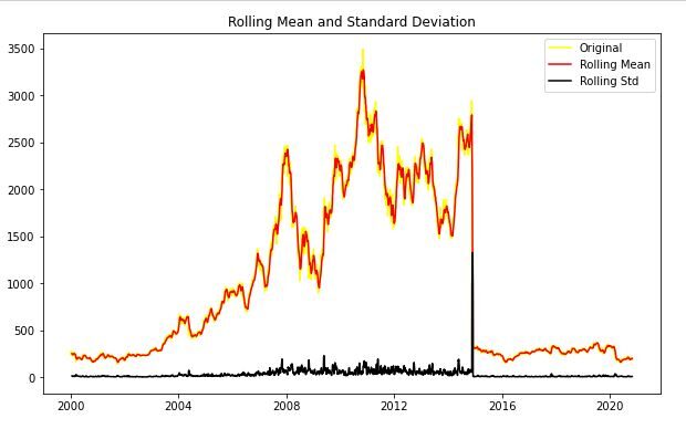
After analysing the above graph, we can see the increasing mean and standard deviation and hence our series is not stationary.
Results of dickey fuller test
Test Statistics                  -1.914523
p-value                           0.325260
No. of lags used                  3.000000
Number of observations used    5183.000000
critical value (1%)              -3.431612
critical value (5%)              -2.862098
critical value (10%)             -2.567067
dtype: float64
We see that the p-value is greater than 0.05 so we cannot reject the Null hypothesis. What's more, test statistics are greater than critical values. so the data is not stationary.
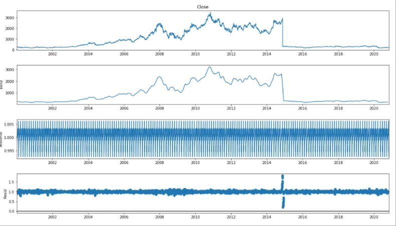
For time series analysis, We separate Trend and Seasonality from the time series.
result = seasonal_decompose(df_close, model="multiplicative", freq = 30)
fig = plt.figure()
fig = result.plot()
fig.set_size_inches(16, 9)
from pylab import rcParams
rcParams['figure.figsize'] = 10, 6
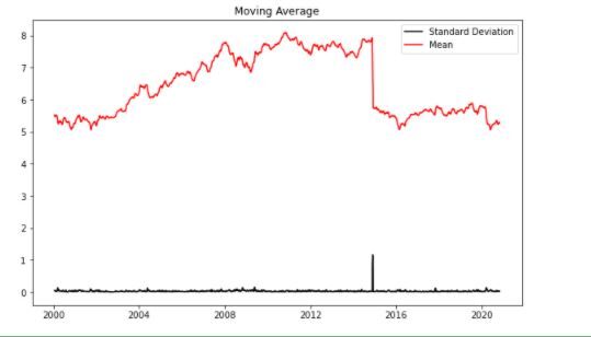
df_log = np.log(sbin['Close'])
moving_avg = df_log.rolling(12).mean()
std_dev = df_log.rolling(12).std()
plt.legend(loc ="best")
plt.title('Moving Average')
plt.plot(std_dev, color ="black", label = "Standard Deviation")
plt.plot(moving_avg, color="red", label = "Mean")
plt.legend()
plt.show()
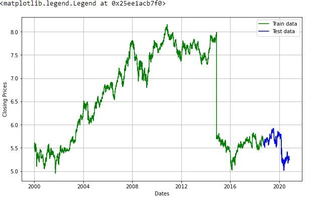
Now we are going to create an ARIMA model and train it with the closing price of the stock in the train data. So let us split the data into trainingTraining is a systematic process designed to improve skills, physical knowledge or abilities. It is applied in various areas, like sport, Education and professional development. An effective training program includes goal planning, regular practice and evaluation of progress. Adaptation to individual needs and motivation are key factors in achieving successful and sustainable results in any discipline.... training and test set and visualize them.
train_data, test_data = df_log[3:int(len(df_log)*0.9)], df_log[int(len(df_log)*0.9):]
plt.figure(figsize=(10,6))
plt.grid(True)
plt.xlabel('Dates')
plt.ylabel('Closing Prices')
plt.plot(df_log, 'green', label="Train data")
plt.plot(test_data, 'blue', label="Test data")
plt.legend()
model_autoARIMA = auto_arima(train_data, start_p=0, start_q=0,
test="adf",       # use adftest to find optimal 'd'
max_p=3, max_q=3, # maximum p and q
m=1,              # frequency of series
d=None,           # let model determine 'd'
seasonal=False,   # No Seasonality
start_P=0,
D=0,
trace=True,
error_action='ignore',
suppress_warnings=True,
stepwise=True)
print(model_autoARIMA.summary())
Performing stepwise search to minimize aic
 ARIMA(0,1,0)(0,0,0)[0] intercept   : AIC=-16607.561, Time=2.19 sec
 ARIMA(1,1,0)(0,0,0)[0] intercept   : AIC=-16607.961, Time=0.95 sec
 ARIMA(0,1,1)(0,0,0)[0] intercept   : AIC=-16608.035, Time=2.27 sec
 ARIMA(0,1,0)(0,0,0)[0]             : AIC=-16609.560, Time=0.39 sec
 ARIMA(1,1,1)(0,0,0)[0] intercept   : AIC=-16606.477, Time=2.77 sec

Best model:  ARIMA(0,1,0)(0,0,0)[0]
Total fit time: 9.079 seconds
                               SARIMAX Results
==============================================================================
Dep. Variable:                      and no. Observations:                 4665
Model:               SARIMAX(0, 1, 0)   Log Likelihood                8305.780
Date:                Tue, 24 Nov 2020   AIC                         -16609.560
Time:                        20:08:50   BIC                         -16603.113
Sample:                             0   HQIC                        -16607.293
                               - 4665
Covariance Type:                  opg
==============================================================================
                 coef    std err          z      P>|With|      [0.025      0.975]
------------------------------------------------------------------------------
sigma2         0.0017   1.06e-06   1566.660      0.000       0.002       0.002
================================================ ================================
Ljung-Box (Q):                       24.41   Jarque-Bera (JB):         859838819.58
Prob(Q):                              0.98   Prob(JB):                         0.00
Heteroskedasticity (H):               7.16   Skew:                           -37.54
Prob(H) (two-sided):                  0.00   Kurtosis:                      2105.12
===================================================================================
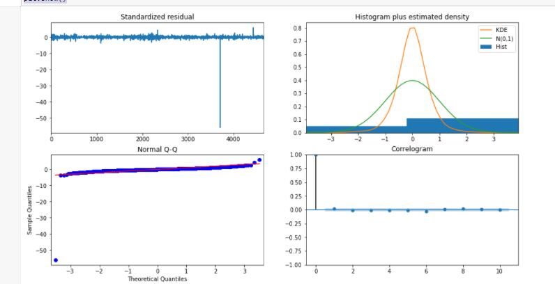
model_autoARIMA.plot_diagnostics(figsize=(15,8))
plt.show()
model = ARIMA(train_data, order=(3, 1, 2))
fitted = model.fit(disp = -1)
print(fitted.summary())
                             ARIMA Model Results
==============================================================================
Dep. Variable:                D.Close   No. Observations:                 4664
Model:                 ARIMA(3, 1, 2)   Log Likelihood                8309.178
Method:                       css-mle S.D.. of innovations              0.041
Date:                Tue, 24 Nov 2020   AIC                         -16604.355
Time:                        20:09:37   BIC                         -16559.222
Sample:                             1   HQIC                        -16588.481

=================================================================================
                    coef    std err          z      P>|With|      [0.025      0.975]
---------------------------------------------------------------------------------
const 8.761e-06      0.001      0.015      0.988      -0.001       0.001
ar.L1.D.Close     1.3689      0.251      5.460      0.000       0.877       1.860
ar.L2.D.Close    -0.7118      0.277     -2.567      0.010      -1.255      -0.168
ar.L3.D.Close     0.0094      0.021      0.445      0.657      -0.032       0.051
ma.L1.D.Close    -1.3468      0.250     -5.382      0.000      -1.837      -0.856
ma.L2.D.Close     0.6738      0.282      2.391      0.017       0.122       1.226
                                    Roots
=============================================================================
                  Real          Imaginary           Modulus         Frequency
-----------------------------------------------------------------------------
AR.1            0.9772           -0.6979j            1.2008           -0.0987
AR.2            0.9772           +0.6979j            1.2008            0.0987
AR.3           74.0622           -0.0000j           74.0622           -0.0000
MA.1            0.9994           -0.6966j            1.2183           -0.0969
MA.2            0.9994           +0.6966j            1.2183            0.0969
-----------------------------------------------------------------------------
# Forecast

fc, I know, conf = fitted.forecast(519, alpha=0.05)  # 95% confidence
fc_series = pd.Series(fc, index=test_data.index)
lower_series = pd.Series(conf[:, 0], index=test_data.index)
upper_series = pd.Series(conf[:, 1], index=test_data.index)
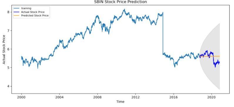
plt.figure(figsize=(12,5), dpi=100)
plt.plot(train_data, label="training")
plt.plot(test_data, color="blue", label="Actual Stock Price")
plt.plot(fc_series, color="orange",label="Predicted Stock Price")
plt.fill_between(lower_series.index, lower_series, upper_series,
                 color="k", alpha=.10)
plt.title('SBIN Stock Price Prediction')
plt.xlabel('Time')
plt.ylabel('Actual Stock Price')
plt.legend(loc ="upper left", fontsize=8)
plt.show()
Conclution
Time series forecasting is really useful when we have to make future decisions or we have to do analysis, we can do it quickly using ARIMA, there are many other models from which we can do time series forecasting, but ARIMA is really easy to understand.
Hope this article helps you and saves you a good amount of time.. Let me know if you have any suggestions..
HAPPY CODING.
Prabhat Pathak (Linkedin profile) is a senior analyst and innovation enthusiast.





