A Simple Overview of Multilayer Perceptron Deep Learning (MLP)

This article was published as part of the Data Science Blogathon.

Introduction

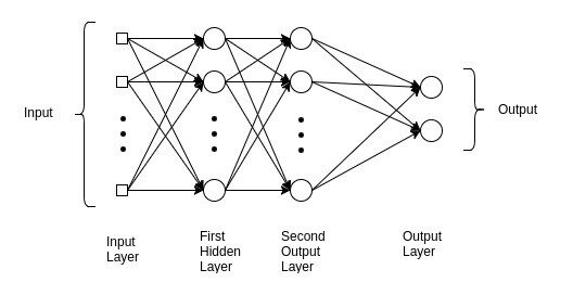
Understanding this network helps us gain insight into the underlying reasons for advanced Deep Learning models. The multilayer perceptron is commonly used in simple regression problems. But nevertheless, MLPs are not ideal for processing patterns with sequential and multidimensional data.

🙄 A multilayer perceptron struggles to remember patterns in sequential data, because of this, requiere una “gran” cantidad de parametersThe "parameters" are variables or criteria that are used to define, measure or evaluate a phenomenon or system. In various fields such as statistics, Computer Science and Scientific Research, Parameters are critical to establishing norms and standards that guide data analysis and interpretation. Their proper selection and handling are crucial to obtain accurate and relevant results in any study or project.... para procesar datos multidimensionales.

MLP, CNN and RNN don't do everything …
Much of your success comes from identifying your goal and choosing a few parameters wisely., What Loss function, Optimizer, Y Regularizer.

We also have data outside the training environment. The role of the regularizer is to ensure that the trained model is generalized to new data.

MNIST data set

Suppose our goal is to create a network to identify numbers based on handwritten digits. For instance, when the input to the network is an image of a number 8, the corresponding forecast must also be 8.
🤷🏻‍♂️ This is a basic classification work with neural networks.

Before analyzing the MLP model, understanding the MNIST dataset is essential. Se utiliza para explicar y validar muchas teorías de deep learningDeep learning, A subdiscipline of artificial intelligence, relies on artificial neural networks to analyze and process large volumes of data. This technique allows machines to learn patterns and perform complex tasks, such as speech recognition and computer vision. Its ability to continuously improve as more data is provided to it makes it a key tool in various industries, from health... porque las 70.000 images it contains are small but rich enough in information;

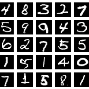
MNIST is a collection of digits ranging from 0 al 9. Tiene un conjunto de trainingTraining is a systematic process designed to improve skills, physical knowledge or abilities. It is applied in various areas, like sport, Education and professional development. An effective training program includes goal planning, regular practice and evaluation of progress. Adaptation to individual needs and motivation are key factors in achieving successful and sustainable results in any discipline.... of 60.000 images and 10.000 tests classified into categories.

Using the MNIST dataset in TensorFlow is simple.

import numpy as e.g
from tensorflow.keras.datasets import mnist
(x_train, y_train), (x_test, y_test) = mnist.load_data()

the mnist.load_data () The method is convenient, since it is not necessary to load the 70.000 images and their labels.

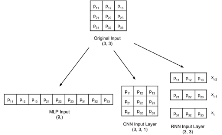
Before entering the Multilayer Perceptron classifier, it is essential to bear in mind that, although the MNIST data consist of two-dimensional tensors, they must be remodeled, según el tipo de input layerThe "input layer" refers to the initial level in a data analysis process or in neural network architectures. Its main function is to receive and process raw information before it is transformed by subsequent layers. In the context of machine learning, Proper configuration of the input layer is crucial to ensure the effectiveness of the model and optimize its performance in specific tasks.....

The shape of a grayscale image is changed from 3 × 3 for MLP input layers, CNN the RNN:

Labels are in the form of digits, of the 0 al 9.

num_labels = len(np.unique(y_train))
print("total de labels:t{}".format(num_labels))
print("labels:ttt{0}".format(np.unique(y_train)))

⚠️ This representation is not suitable for the forecast layer that generates probability by class. The most suitable format is one-hot, a vector of 10 dimensions as all values 0, excepto el indexThe "Index" It is a fundamental tool in books and documents, which allows you to quickly locate the desired information. Generally, it is presented at the beginning of a work and organizes the contents in a hierarchical manner, including chapters and sections. Its correct preparation facilitates navigation and improves the understanding of the material, making it an essential resource for both students and professionals in various areas.... de clase. For instance, if the label is 4, the equivalent vector is [0,0,0,0, 1, 0,0,0,0,0].

En Deep Learning, los datos se almacenan en un tensorTensors are mathematical structures that generalize concepts such as scalars and vectors. They are used in various disciplines, including physics, Engineering and Machine Learning, to represent multidimensional data. A tensor can be visualized as a multi-dimensional matrix, which allows complex relationships between different variables to be modeled. Their versatility and ability to handle large volumes of information make them fundamental tools in data analysis and processing..... The term tensor applies to a scalar tensor (tensor 0D), vector (tensor 1D), headquarters (two-dimensional tensor) Y tensor multidimensionalLos tensores multidimensionales son estructuras matemáticas que generalizan la noción de escalares, vectores y matrices a dimensiones superiores. Se utilizan ampliamente en campos como la física, la ingeniería y el aprendizaje automático, permitiendo representar y manipular datos complejos de manera eficiente. Su capacidad para almacenar información en múltiples dimensiones facilita el análisis y la modelización de fenómenos reales, contribuyendo a avances en diversas disciplinas científicas y tecnológicas.....

#converter em one-hot
from tensorflow.keras.utils import to_categorical
y_train = to_categorical(y_train)
y_test = to_categorical(y_test)

Our model is an MLP, so your inputs must be a 1D tensor. as such, x_train and x_test must be transformed into [60,000, 2828] Y [10,000, 2828],

In sum, the size of -1 means allowing the library to calculate the correct dimension. In the case of x_train, it is 60.000.

image_size = x_train.shape[1] 
input_size = image_size * image_size

print("x_train:t{}".format(x_train.shape))
print("x_test:Tt{}n".format(x_test.shape))

x_train = np.reshape(x_train, [-1, input_size])
x_train = x_train.astype('float32') / 255

x_test = np.reshape(x_test, [-1, input_size])
x_test = x_test.astype('float32') / 255

print("x_train:t{}".format(x_train.shape))
print("x_test:Tt{}".format(x_test.shape))

OUTPUT:

x_train:	(60000, 28, 28)
x_test:		(10000, 28, 28)

x_train:	(60000, 784)
x_test:		(10000, 784)

Building the model

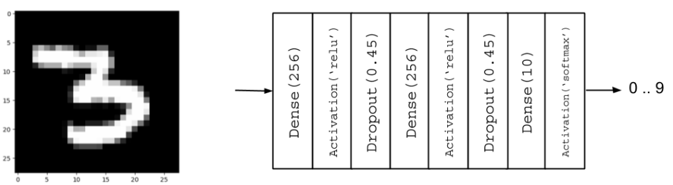
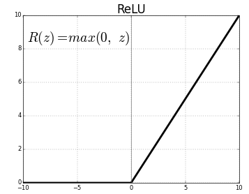
from tensorflow.keras.models import Sequential
from tensorflow.keras.layers import Dense, Activation, Dropout

# Parameters
batch_size = 128 # It is the sample size of inputs to be processed at each training stage. 
hidden_units = 256
dropout = 0.45

# Nossa  MLP com ReLU e Dropout 
model = Sequential()

model.add(Dense(hidden_units, input_dim=input_size))
model.add(Activation('relu'))
model.add(Dropout(dropout))

model.add(Dense(hidden_units))
model.add(Activation('relu'))
model.add(Dropout(dropout))

model.add(Dense(num_labels))

Regularization

A neural network tends to memorize its training data, especially if it contains more than enough capacity. In this case, network fails catastrophically when subjected to test data.

This is the classic case in which the network fails to generalize (OverfittingOverfitting, or overfitting, It's a phenomenon in machine learning where a model fits too closely with the training data, capturing irrelevant noise and patterns. This results in poor performance on unseen data, since the model loses generalization capacity. To mitigate overfitting, Techniques such as regularization can be used, cross-validation and reduction of model complexity.... / UnderfittingEl underfitting es un problema común en el aprendizaje automático que ocurre cuando un modelo es demasiado simple para capturar la complejidad de los datos. Esto se traduce en un rendimiento deficiente tanto en el conjunto de entrenamiento como en el de prueba. Las causas del underfitting pueden incluir un modelo inadecuado, características irrelevantes o insuficientes datos. In order to solve it, se puede optar por modelos más complejos o mejorar la calidad...). To avoid this trend, the model uses a regulating layer. Leave.

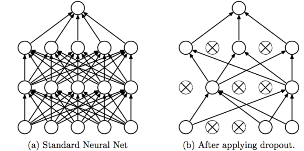
The idea of Dropout is simple. Given a discard rate (in our model, we set = 0,45), the layer randomly removes this fraction of units.

For instance, whether the first layer has 256 units, after abandonment is applied (0.45), solo (1 – 0.45) * 255 = 140 units will participate in the next layer

Attrition makes neural networks more robust for unforeseen input data, because the network is trained to predict correctly, even if some units are absent.

⚠️ Abandonment only participates in “play” 🤷🏻 ♂️ during training.

Activation

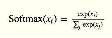
The Output layerThe "Output layer" is a concept used in the field of information technology and systems design. It refers to the last layer of a software model or architecture that is responsible for presenting the results to the end user. This layer is crucial for the user experience, since it allows direct interaction with the system and the visualization of processed data.... has 10 units, followed by a softmax activation function. The 10 units correspond to the 10 possible tags, classes or categories.

Softmax activation can be expressed mathematically, according to the following equation:

model.add(Activation('softmax'))
model.summary()

OUTPUT:

Model: "sequential"
_________________________________________________________________
Layer (type)                 Output Shape              Param #   
=================================================================
dense (Dense)                (None, 256)               200960    
_________________________________________________________________
activation (Activation)      (None, 256)               0         
_________________________________________________________________
dropout (Dropout)            (None, 256)               0         
_________________________________________________________________
dense_1 (Dense)              (None, 256)               65792     
_________________________________________________________________
activation_1 (Activation)    (None, 256)               0         
_________________________________________________________________
dropout_1 (Dropout)          (None, 256)               0         
_________________________________________________________________
dense_2 (Dense)              (None, 10)                2570      
_________________________________________________________________
activation_2 (Activation)    (None, 10)                0         
=================================================================
Total params: 269,322
Trainable params: 269,322
Non-trainable params: 0
_________________________________________________________________

Viewing models

Improvement

The purpose of Optimization is to minimize the loss function. The idea is that if the loss is reduced to an acceptable level, the model indirectly learned the function that assigns inputs to outputs. Performance metrics are used to determine if your model has learned.

model.compile(loss="categorical_crossentropy", optimizer="adam", metrics=['accuracy'])

📌 Given our training set, la elección de la Loss functionThe loss function is a fundamental tool in machine learning that quantifies the discrepancy between model predictions and actual values. Its goal is to guide the training process by minimizing this difference, thus allowing the model to learn more effectively. There are different types of loss functions, such as mean square error and cross-entropy, each one suitable for different tasks and..., the optimizer and the regularizer, we can start training our model.

model.fit(x_train, y_train, epochs=20, batch_size=batch_size)

OUTPUT:

Epoch 1/20
469/469 [==============================] - 1s 3ms/step - loss: 0.4230 - accuracy: 0.8690

....

Epoch 20/20
469/469 [==============================] - 2s 4ms/step - loss: 0.0515 - accuracy: 0.9835

Evaluation

In this point, our MNIST digit classifier model is complete. Your performance evaluation will be the next step in determining whether the trained model will present a suboptimal solution.

_, acc = model.evaluate(x_test,
                        y_test,
                        batch_size=batch_size,
                        verbose=0)
print("nAccuracy: %.1f%%n" % (100.0 * acc))

OUTPUT:

Accuracy: 98.4%

to be continue…

Related