
This article was published as part of the Data Science Blogathon
Introduction
VGG- Network is a model of red neuronal convolucionalConvolutional Neural Networks (CNN) are a type of neural network architecture designed especially for data processing with a grid structure, as pictures. They use convolution layers to extract hierarchical features, which makes them especially effective in pattern recognition and classification tasks. Thanks to its ability to learn from large volumes of data, CNNs have revolutionized fields such as computer vision.. proposed by K. Simonyan y A. Zisserman in the article “Very deep convolutional networks for large-scale image recognition” [1]. This architecture achieved test accuracy between the 5 best of 92,7% on ImageNet, that has more than 14 million images belonging to 1000 lessons.
It is one of the well-known architectures in the field of deep learningDeep learning, A subdiscipline of artificial intelligence, relies on artificial neural networks to analyze and process large volumes of data. This technique allows machines to learn patterns and perform complex tasks, such as speech recognition and computer vision. Its ability to continuously improve as more data is provided to it makes it a key tool in various industries, from health.... Replace large kernel size filters with 11 Y 5 in the first and second layer, respectively, showed improvement over AlexNet architecture, with multiple kernel size filters from 3 × 3 one after another. It was trained for weeks and was using NVIDIA Titan Black GPU.
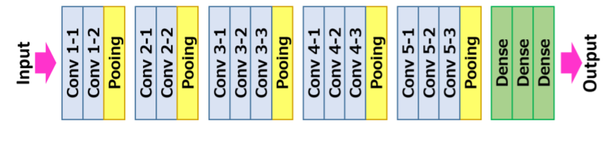
VGG16 architecture
The input to the red neuronalNeural networks are computational models inspired by the functioning of the human brain. They use structures known as artificial neurons to process and learn from data. These networks are fundamental in the field of artificial intelligence, enabling significant advancements in tasks such as image recognition, Natural Language Processing and Time Series Prediction, among others. Their ability to learn complex patterns makes them powerful tools.. convolution is a fixed-size RGB image 224 × 224. The only pre-processing it does is subtract the average RGB values, which are computed from the dataset of trainingTraining is a systematic process designed to improve skills, physical knowledge or abilities. It is applied in various areas, like sport, Education and professional development. An effective training program includes goal planning, regular practice and evaluation of progress. Adaptation to individual needs and motivation are key factors in achieving successful and sustainable results in any discipline...., of each pixel.
Later, the image runs through a stack of convolutional layers (Conv.), Where there are filters with a very small receptive field that is 3 × 3, which is the smallest size to capture the notion of left / right, up / down, and central part.
In one of the configurations, also uses convolution filters 1 × 1, which can be observed as a linear transformation of the input channels followed by non-linearity. Convolutional strides are fixed at 1 pixel; the spatial padding of the input of the convolutional coverThe Convolutional Layer, fundamental in convolutional neural networks (CNN), It is mainly used for data processing with grid-like structures, as pictures. This layer applies filters that extract relevant features, such as edges and textures, allowing the model to recognize complex patterns. Its ability to reduce the dimensionality of data and maintain essential information makes it a key tool in computer vision tasks.. is such that the resolutionThe "resolution" refers to the ability to make firm decisions and meet set goals. In personal and professional contexts, It involves defining clear goals and developing an action plan to achieve them. Resolution is critical to personal growth and success in various areas of life, as it allows you to overcome obstacles and keep your focus on what really matters.... spatial dimensions are maintained after convolution, namely, the filling is 1 pixel for 3 × 3 Conv. covers.
Later, spatial clustering is carried out by five layers of maximum clustering, 16 that follow some of the Conv. covers, but not all Conv. layers are followed by maximum grouping. This maximum grouping is done in a window of 2 × 2 pixels, with step 2.
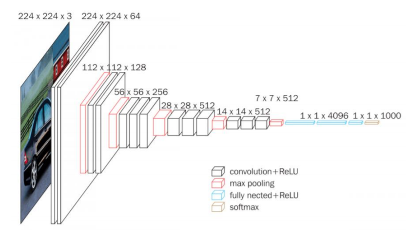
The architecture contains a stack of convolutional layers that have a different depth in different architectures that are followed by three Fully-Connected layers (FC): the first two FC have 4096 channels each and the third FC performs a classification of 1000 routes and therefore contains 1000 channels which is one for each class.
The last layer is the soft-max layer. The configuration of the fully connected layers is similar in all networks.
All hidden layers are equipped with rectification (resumeThe ReLU activation function (Rectified Linear Unit) It is widely used in neural networks due to its simplicity and effectiveness. Defined as ( f(x) = max(0, x) ), ReLU allows neurons to fire only when the input is positive, which helps mitigate the problem of gradient fading. Its use has been shown to improve performance in various deep learning tasks, making ReLU an option...) nonlinear. What's more, here one of the networks contains NormalizationStandardization is a fundamental process in various disciplines, which seeks to establish uniform standards and criteria to improve quality and efficiency. In contexts such as engineering, Education and administration, Standardization makes comparison easier, interoperability and mutual understanding. When implementing standards, cohesion is promoted and resources are optimised, which contributes to sustainable development and the continuous improvement of processes.... local response (LRN), such normalization does not improve performance on the trained dataset, but its use leads to higher memory consumption and calculation time.
Architecture Summary:
• The input to the model is a fixed-size RGB image 224 × 224224 × 224
• Preprocessing consists of subtracting the mean of the RGB value of the training set from each pixel
• Convolutional layers 17
– Fixed stride to 1 pixel
– the filling is 1 pixel for 3 × 33 × 3
• Spatial grouping layers
– This layer does not count towards the depth of the web by convention
– Spatial grouping is done using maximum grouping layers
– the window size is 2 × 22 × 2
– Stride set to 2
– Convnets used 5 maximum grouping layers
• Fully connected layers:
• 1º: 4096 (resume).
▪ 2do: 4096 (resume).
▪ 3º: 1000 (Softmax).
Architecture configuration
The following figure"Figure" is a term that is used in various contexts, From art to anatomy. In the artistic field, refers to the representation of human or animal forms in sculptures and paintings. In anatomy, designates the shape and structure of the body. What's more, in mathematics, "figure" it is related to geometric shapes. Its versatility makes it a fundamental concept in multiple disciplines.... contains the VGG network convolutional neural network configuration with
next layers:
• VGG-11
• VGG-11 (LRN)
• VGG-13
• VGG-16 (Conv1)
• VGG-16
• VGG-19
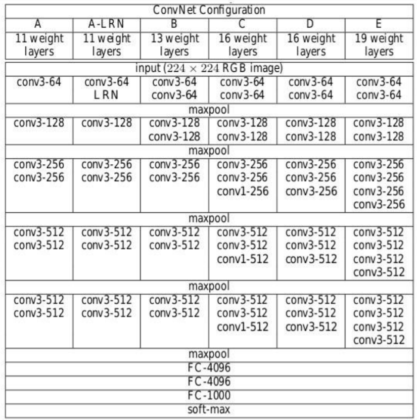
Source: “Very deep convolutional networks for large-scale image recognition”
Convolutional neural network configurations are mentioned above one per column.
Then, networks are referred to by their names (A - E). All configurations follow the traditional design and differ only in depth: of 11 weight layers in network A which are 8 Conv. Y 3 layers FC a 19 weight layers in the E network which is 16 Conv. Y 3 FC layers. The width of each conv. layer is the number of channels is quite small, that starts from 64 in the first layer and then continues to increase by a factor of 2 after each layer of maximum grouping until reaching 512.
The number of parametersThe "parameters" are variables or criteria that are used to define, measure or evaluate a phenomenon or system. In various fields such as statistics, Computer Science and Scientific Research, Parameters are critical to establishing norms and standards that guide data analysis and interpretation. Their proper selection and handling are crucial to obtain accurate and relevant results in any study or project.... for each configuration is described below. Although it has great depth, the number of weights in the networks is not greater than the number of weights in a shallower network with higher conv. layer widths and receptive fields

Training
• The Loss functionThe loss function is a fundamental tool in machine learning that quantifies the discrepancy between model predictions and actual values. Its goal is to guide the training process by minimizing this difference, thus allowing the model to learn more effectively. There are different types of loss functions, such as mean square error and cross-entropy, each one suitable for different tasks and... is a multinomial logistic regression
• The learning algorithm is gradient descent gradientGradient is a term used in various fields, such as mathematics and computer science, to describe a continuous variation of values. In mathematics, refers to the rate of change of a function, while in graphic design, Applies to color transition. This concept is essential to understand phenomena such as optimization in algorithms and visual representation of data, allowing a better interpretation and analysis in... stochastic (SGD) mini-batch based on momentum backspread.
· The lot size was 256
· The impulse was 0,9
• RegularizationRegularization is an administrative process that seeks to formalize the situation of people or entities that operate outside the legal framework. This procedure is essential to guarantee rights and duties, as well as to promote social and economic inclusion. In many countries, Regularization is applied in migratory contexts, labor and tax, allowing those who are in irregular situations to access benefits and protect themselves from possible sanctions....
· L2 weight decay (the penalty multiplier was 0,0005)
· Dropout for the first two fully connected layers is set to 0.5
• Learning rate
· initial: 0.01
· When the accuracy of the validation set stopped improving, se reduce a 10.
• Although it has a greater number of parameters and also depth compared to Alexnet, CNN required fewer times for the loss function to converge due to
· Small convolutional grains and more regularization due to great depth.
· Pre-initialization of certain layers.
• Training image size
· S is the smallest side of the isotopically rescaled image
· Two approaches to establishing S
▪ Fix S, known as single scale training
▪ Here S = 256 y S = 384
▪ Vary S, known as multi-scale training
▪ S de [Smin, Smax] where Smin = 256, Smax = 512
– Later 224 × 224224 × 224
Image was randomly cropped from SGD iteration rescaled image.
Key features
• VGG16 has a total of 16 layers that have some weights.
• Only convolution and grouping layers are used.
• Always use a core of 3 x 3 for convolution. 20
• Size 2 × 2 maximum pool.
• 138 million parameters.
• Trained in ImageNet data.
• Has an accuracy of 92,7%.
• Another version that is VGG 19, has a total of 19 layers with weights.
• It is a very good deep learning architecture for benchmarking on any particular task.
• Pre-trained networks for VGG are open source, so they can be commonly used for various kinds of applications.
Implementemos VGG Net
First, let's create filter mapping for each version of the VGG network. Please refer to the configuration image above for the number of filters. Namely, create a dictionary for the version with a key named VGG11, VGG13, VGG16, VGG19 and create a list according to the number of filters in each version respectively. Here “M” in the list it is known as Maxpool operation.
import torch
import torch.nn as nn
VGG_types = {
"VGG11": [64, "M", 128, "M", 256, 256, "M", 512, 512, "M", 512, 512, "M"],
"VGG13": [64, 64, "M", 128, 128, "M", 256, 256, "M", 512, 512, "M", 512, 512, "M"],
"VGG16": [64,64,"M",128,128,"M",256,256,256,"M",512,512,512,"M",512,512,512,"M",],
"VGG19": [64,64,"M",128,128,"M",256,256,256,256,"M",512,512,512,512,
          "M",512,512,512,512,"M",],}
Create a variableIn statistics and mathematics, a "variable" is a symbol that represents a value that can change or vary. There are different types of variables, and qualitative, that describe non-numerical characteristics, and quantitative, representing numerical quantities. Variables are fundamental in experiments and studies, since they allow the analysis of relationships and patterns between different elements, facilitating the understanding of complex phenomena.... global to mention the version of the architecture. Then create a class called VGG_net with inputs like in_channels and num_classes. Takes inputs as a number of image channels and the number of output classes.
Initialize sequential layers, namely, in the sequence, Linear layer–> ReLU–> Skip.
Then create a function called create_conv_layers which takes the VGGnet architecture configuration as input, which is the list that we created previously for different versions. When he meets the letter “M” from the list above, perform the MaxPool2d operation.
VGGType = "VGG16"
class VGGnet(nn.Module):
    def __init__(self, in_channels=3, num_classes=1000):
        super(VGGnet, self).__init__()
        self.in_channels = in_channels
        self.conv_layers = self.create_conv_layers(VGG_types[VGGType])
self.fcs = nn.Sequential(
nn.Linear(512 * 7 * 7, 4096),
nn.ReLU(),
nn.Dropout(p=0.5),
nn.Linear(4096, 4096),
nn.ReLU(),
nn.Dropout(p=0.5),
nn.Linear(4096, num_classes),
)

def forward(self, x):
x = self.conv_layers(x)
x = x.reshape(x.shape[0], -1)
x = self.fcs(x)
return x

def create_conv_layers(self, architecture):
layers = []
in_channels = self.in_channels

for x in architecture:
if type(x) == int:
out_channels = x

layers += [
nn.Conv2d(
in_channels=in_channels,
out_channels=out_channels,
kernel_size=(3, 3),
stride=(1, 1),
padding=(1, 1),
),
nn.BatchNorm2d(x),
nn.ReLU(),
]
in_channels = x
elif x == "M":
layers += [nn.MaxPool2d(kernel_size=(2, 2), stride=(2, 2))]

return nn.Sequential(*layers)
Once this is done, write a little test code to check if our implementation is working fine.
In the following test code, the number of classes given is 500.
if __name__ == "__main__":
    device = "miracles" if torch.cuda.is_available() else "cpu"
    model = VGGnet(in_channels=3, num_classes=500).to(device)
    # print(model)
    x = torch.randn(1, 3, 224, 224).to(device)
    print(model(x).shape)
The output should be like this:
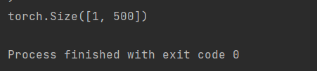
If you want to see the network architecture, you can uncomment the to print (model) above code declaration. You can also try different versions by changing the VGG versions in the VGGType variable.
The full code can be accessed here:
https://github.com/BakingBrains/Deep_Learning_models_implementation_from-scratch_using_pytorch_/blob/main/VGG.py
[1]. K. Simonyan y A. Zisserman: Very deep convolutional networks for large-scale image recognition, april of 2015, DOI: https://arxiv.org/pdf/1409.1556.pdf
Thanks
The media shown in this article is not the property of DataPeaker and is used at the author's discretion.





