
Introduction
Data is everywhere around us, in spreadsheets, on various social media platforms, on survey forms and more. The cleaning process, transformation, interpretation, analysis and visualization of this data to extract useful information and obtain valuable information to make more effective business decisions is called Data Analysis.
Data analysis can be organized into 6 types
- Exploratory analysis
- Descriptive analysis
- Inferential analysis
- Predictive analytics
- Causal analysis
- Mechanistic analysis
Here, we will dive deep into Exploratory analysis,
Exploratory analysis
Preliminary data analysis to discover relationships between measures in the data and to gain insight into trends, patterns and relationships between various entities present in the dataset with the help of statistics and visualization tools is called Exploratory Data Analysis (EDA). .
Exploratory data analysis is cross-classified in two different ways in which each method is graphical or non-graphical. And later, each method is univariate, bivariate or multivariate.
Univariate analysis
Uni means one and variable means variable, so in the univariate analysis, there is only one reliable variable. The goal of univariate analysis is to derive the data, define and summarize them and analyze the pattern present in them. In a data set, explore each variable separately. It is possible for two types of variables: categorical and numerical.
Some patterns that can be easily identified with univariate analysis are Central trend (media, fashion and medium), Dispersion (rank, variance), Quartiles (interquartile range) and standard deviation.
Univariate data can be described by:
Ø Frequency distribution tables
The frequency distribution table reflects the frequency with which an occurrence has occurred in the data. Gives a brief idea of the data and makes it easy to find patterns.
Example:
The list of IQ scores is: 118, 139, 124, 125, 127, 128, 129, 130, 130, 133, 136, 138, 141, 142, 149, 130, 154.
| IQ range | Number |
| 118-125 | 3 |
| 126-133 | 7 |
| 134-141 | 4 |
| 142-149 | 2 |
| 150-157 | 1 |
Ø Bar graph
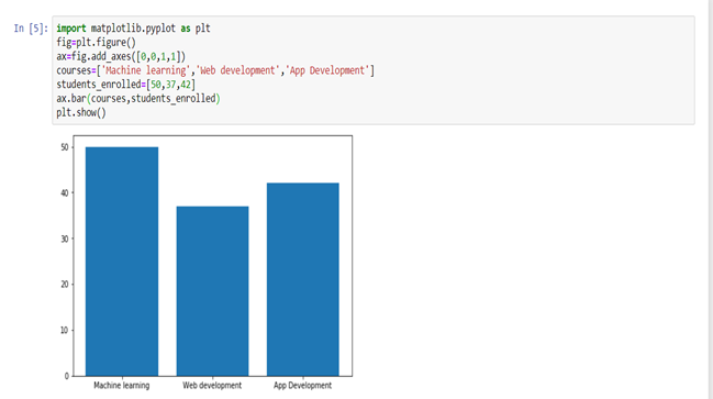
The bar chart is very convenient when comparing categories of data or different groups of data. Helps track changes over time. It is better for displaying discrete data.
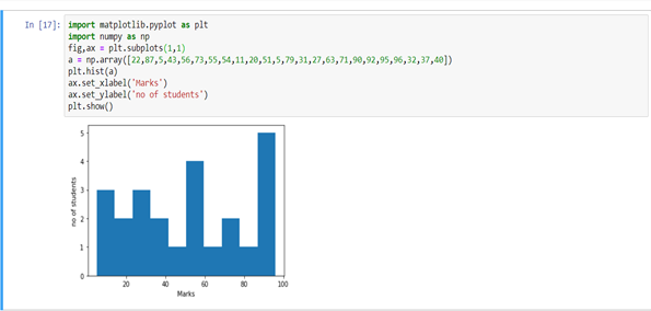
Ø HistogramasHistograms are graphical representations that show the distribution of a dataset. They are constructed by dividing the range of values into intervals, O "Bins", and counting how much data falls in each interval. This visualization allows you to identify patterns, trends and variability of data effectively, facilitating statistical analysis and informed decision-making in various disciplines....
Histograms are similar to bar charts and show the same categorical variables in the data category. Histograms display these categories as containers that indicate the number of data points in a range.. It is better for visualizing continuous data.
Ø Pie charts
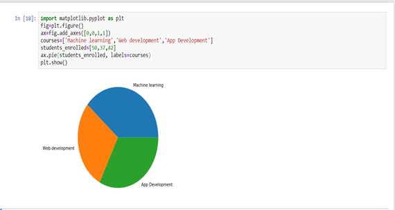
Pie charts are primarily used to understand how a group is divided into smaller parts. The whole cake represents the 100 percent and servings denote the relative size of that particular category.
Ø Frequency polygons
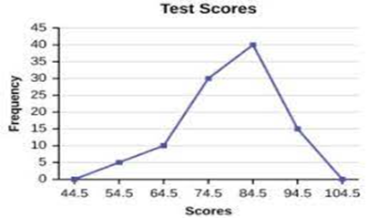
Similar to histograms, a frequency polygon is used to compare data sets or show the cumulative frequency distribution.
Bivariate analysis
Bi means two and variable means variable, hence here are two variables. The analysis is related to the cause and the relationship between the two variables. There are three types of bivariate analysis.
Bivariate analysis of two numerical variables (Numerical-Numeric)
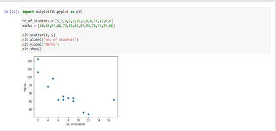
Ø Scatter plotA scatter plot is a visual representation that shows the relationship between two numerical variables using points on a Cartesian plane. Each axis represents a variable, and the location of each point indicates its value in relation to both. This type of chart is useful for identifying patterns, Correlations and trends in the data, facilitating the analysis and interpretation of quantitative relationships....
A The scatter plot represents individual data using points. These charts make it easy to see if two variables are related to each other.. The resulting pattern indicates the type (linear or non-linear) and the strength of the relationship between two variables.
Ø Linear correlation
Lineal Correlation represents the strength of a linear relationship between two numeric variables. If there is no correlation between the two variables, there is no tendency to change along with the values of the second quantity.
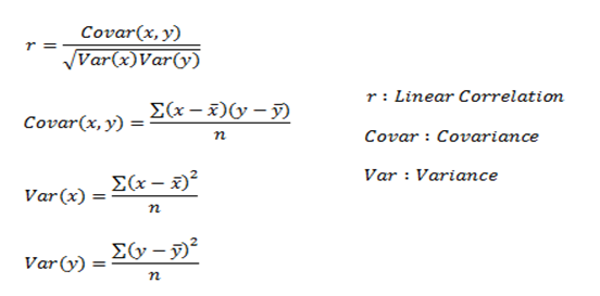
Here, r measures the strength of a linear relationship and is always between -1 Y 1 where -1 denotes a perfect negative linear correlation and +1 denotes a perfect positive linear correlation and zero indicates no linear correlation.
Bivariate analysis of two categorical variables (Categorical-Categorical)
Ø Chi-square test
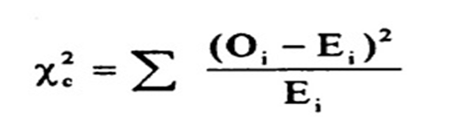
The chi-square test is used to determine the association between categorical variables. It is calculated based on the difference between the expected frequencies and the observed frequencies in one or more categories of the frequency table. A probability of zero indicates a complete dependence between two categorical variables and a probability of one indicates that two categorical variables are completely independent..
Here, the subscript c indicates the degrees of freedom, O indicates the observed value and E indicates the expected value.
Bivariate analysis of a variableIn statistics and mathematics, a "variable" is a symbol that represents a value that can change or vary. There are different types of variables, and qualitative, that describe non-numerical characteristics, and quantitative, representing numerical quantities. Variables are fundamental in experiments and studies, since they allow the analysis of relationships and patterns between different elements, facilitating the understanding of complex phenomena.... numerical and a categorical (Numerical-Categorical)
Ø Z test and t test
The Z and T tests are important to calculate whether the difference between a sample and a population is substantial..
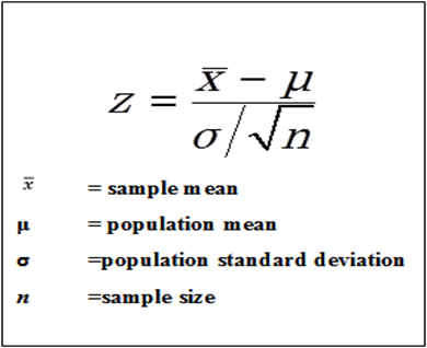
If the probability of Z is small, the difference between the two averages is more significant.
Test T
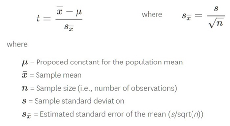
If the sample size is large enough, we use a Z test, and for a small sample size, we use a T test.
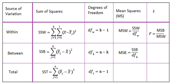
Ø VARIANCE ANALYSIS (ANOVA)
The ANOVA test is used to determine if there is a significant difference between the means of more than two groups that are statistically different from each other.. This analysis is appropriate for comparing the means of a numerical variable for more than two categories of a categorical variable..
Analisis multivariable
Multivariate analysis is necessary when more than two variables must be analyzed simultaneously. It is a tremendously difficult task for the human brain to visualize a relationship between 4 variables in a graph and, Thus, multivariate analysis is used to study more complex data sets. Types of multivariate analysis include cluster analysis, factorial analysis, multiple regression analysis, principal component analysis, etc. There are more than 20 different ways to perform multivariate analysis and which one to choose depends on the type of data and the end goal to be achieved. The most common forms are:
Ø Cluster analysis
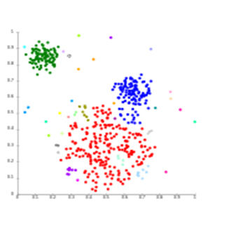
Cluster analysis classifies different objects into clusters so that the similarity between two objects of the same group is maximum and minimum otherwise. Used when the rows and columns of the The data table represents the same units and the measure represents the distance or similarity.
Ø Principal component analysis (PCA)
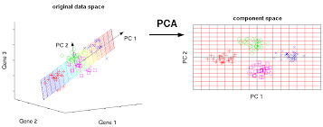
Principal component analysis (o PCA) used to reduce the dimensionality of a data table with a large number of interrelated measures. Here, the original variables become a new set of variables, which are known as the “Main components” of principal component analysis.
PCA is used for the data set showing multicollinearity. Although least squares estimates are biased, the distance between the variances and their real value can be really large. Then, PCA adds some bias and reduces the standard error for the regression model.
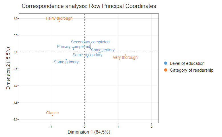
Ø Correspondence analysis
Correspondence analysis using data from a contingency table shows the relative relationships between two different groups of variables. A contingency table is a 2D table with rows and columns as groups of variables.
Conclution
Hope you now have a better understanding of the various techniques used in univariate analysis, bivariate and multivariate.
The media shown in this article is not the property of DataPeaker and is used at the author's discretion.





