
This post was released as part of the Data Science Blogathon
Introduction
to better understand your data, which helps in further data preprocessing. And data visualization is key, as it streamlines the exploratory data analysis procedure and analyzes the data easily through wonderful charts and graphs.

Table of Contents
- Data visualization
- Exploratory data analysis
- Univariate analysis
- Categorical data
- Numerical data
- Bivariate analysis / multivariate
- Numeric and numeric
- Numerical and categorical
- Categorical and categorical
- Final notes
Data visualization
Data visualization represents text or numeric data in a visual format, which facilitates the understanding of the information expressed by the data. U.S, the humans, we remember images more easily than readable text, so Python provides us with various libraries for data visualization like matplotlib, seaborn, plotly, etc. In this tutorial, we will use Matplotlib and seaborn to perform various techniques to explore data using various plots.
Exploratory data analysis
Create hypotheses, testing various business assumptions while dealing with any machine learning problem statement is very important and this is what EDA helps to achieve. There are several tools and techniques to understand your data, and the basic need is that you must have the knowledge of Numpy for math operations and Pandas for data manipulation.
We will use a very popular Titanic dataset that everyone is familiar with and can download from here.
Now let's start exploring data and studying different data visualization charts with different types of data.. And to demonstrate some of the techniques, We will also use a built-in dataset from seaborn as tip data that explains the tips that each waiter receives from different customers..
let's start by importing libraries and loading data
import numpy as np
import pandas pd
import matplotlib.pyplot as plt
import seaborn as sns
from seaborn import load_dataset
#titanic dataset
data = pd.read_csv("titanic_train.csv")
#tips dataset
tips = load_dataset("tips")
Univariate analysis
Univariate analysis is the simplest form of analysis where we explore a single variableIn statistics and mathematics, a "variable" is a symbol that represents a value that can change or vary. There are different types of variables, and qualitative, that describe non-numerical characteristics, and quantitative, representing numerical quantities. Variables are fundamental in experiments and studies, since they allow the analysis of relationships and patterns between different elements, facilitating the understanding of complex phenomena..... Univariate analysis is performed to describe the data in a better way. we perform univariate analyzes of numerical and categorical variables differently because the plot uses different graphs.
Categorical data
A variable that has text-based information is known as categorical variables. let's look at several graphs that we can use to visualize categorical data.
1) CountPlot
Countplot is simply a graph of frequency count in the form of bar graphicThe bar chart is a visual representation of data that uses rectangular bars to show comparisons between different categories. Each bar represents a value and its length is proportional to it. This type of chart is useful for visualizing and analyzing trends, facilitating the interpretation of quantitative information. It is widely used in various disciplines, such as statistics, Marketing and research, due to its simplicity and effectiveness..... Plot the count for each category on a separate bar. When we use the count function of pandas values in any column, is the same visual form of the count value function. Our data destination variable survives and is categorical, so let's draw a tally graph of this.
sns.countplot(data['Survived'])
plt.show()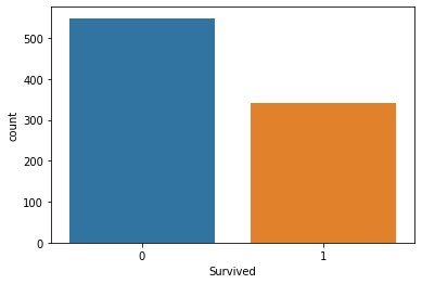
2) pie chartThe pie chart, Also known as pie chart, is a visual representation that shows the proportion of different parts to a whole. It is commonly used in statistics to illustrate the distribution of categorical data. Each section of the chart represents a percentage of the total, making it easier to compare between categories. Its clear and concise design makes it an effective tool for the presentation of quantitative information....
The pie chart is also the same as the counting chart, it only gives you additional information about the percentage of presence of each category in the data, which means which category gets the amount of weighting in the data. Let's look at the Sex column, what is the percentage of male and female members traveling.
data['Sex'].value_counts().plot(kind="pie", autopct="%.2f")
plt.show()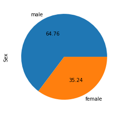
Numerical data
Numerical data analysis is essential because understanding the distribution of variables helps to further process the data. Most of the time you will find a lot of inconsistency with the numerical data, therefore explore numeric variables.
1) Histogram
A histogram is a distribution graph of numeric column values. It just creates bins in various ranges of values and plots them where we can visualize how the values are distributed. We can see where more values are found, as positive, negative or in the center (media). Let's take a look at the Age column.
plt.hist(data['Age'], bins=5)
plt.show()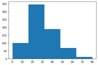
2) Distplot
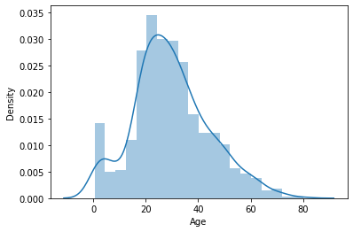
Distplot is also known as the second histogram because it is a slightly enhanced version of the histogram.. Distplot gives us a KDE (Kernel density estimation) about histogram explaining PDF (Probability density function), which means what is the probability that each value occurs in this column. If you have studied statistics before, you should definitely know the PDF function.
sns.distplot(data['Age'])
plt.show()
3) Box plot
Boxplot is a very interesting plot that simply plots a summary of 5 numbers. For a summary of 5 numbers, we need to describe some terms.
- MedianThe median is a statistical measure that represents the central value of a set of ordered data. To calculate it, the data is organized from lowest to highest and the number in the middle is identified. If there are an even number of observations, the two core values are averaged. This indicator is especially useful in asymmetric distributions, since it is not affected by extreme values....: mean value in series after sorting
- Percentile: gives whatever number is the number of values present before this percentile as, as an example, 50 below percentile 25, so it explains the total of 50 values that are below the percentile 25
- Minimum and maximum: these are not minimum and maximum values, Rather, they describe the lower and upper limit of the standard deviation that is calculated using the interquartile range. (IQR).
IQR = Q3 - Q1
Lower_boundary = Q1 - 1.5 * IQR
Upper_bounday = Q3 +  1.5 * IQR
Here Q1 and Q3 are the first quantile (percentile 25) and the third quantile (percentile 75)
Bivariate analysis / multivariate
We have studied several plots to explore unique numerical and categorical data. Bivariate Analysis is used when we have to explore the link between 2 different variables and we have to do it because, in the end, our main task is to explore the linkage between the variables to build a powerful model. And when we analyze more than 2 variables together, known as multivariate analysis. we will work on different graphs for Bivariate as well as Multivariate Analysis.
Numeric and numeric
First, let's explore the graphs when both variables are numeric.
1) Scatter plotA scatter plot is a visual representation that shows the relationship between two numerical variables using points on a Cartesian plane. Each axis represents a variable, and the location of each point indicates its value in relation to both. This type of chart is useful for identifying patterns, Correlations and trends in the data, facilitating the analysis and interpretation of quantitative relationships....
Plotting the link between two scatter plots of numeric variables is a simple graph to do. Let's look at the link between the total bill and the tip provided through a Dispersion diagramThe scatter plot is a graphical tool used in statistics to visualize the relationship between two variables. It consists of a set of points in a Cartesian plane, where each point represents a pair of values corresponding to the variables analyzed. This type of chart allows you to identify patterns, Trends and possible correlations, facilitating data interpretation and decision-making based on the visual information presented.....
sns.scatterplot(tips["total_bill"], tips["tip"])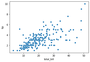
Multivariate analysis with scatter plot
we can also graph relationships of 3 variables or 4 variables with a scatter plot. Suppose we want to find the separate ratio of men and women with the total bill and tip provided.
sns.scatterplot(tips["total_bill"], tips["tip"], hue=tips["sex"])
plt.show()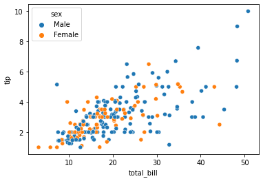
We can also see multivariate analysis of 4 variables with scatterplots using style arguments. Suppose now, along with gender, I also want to know if the client was a smoker or not so that we can do this.
sns.scatterplot(tips["total_bill"], tips["tip"], hue=tips["sex"], style=tips['smoker'])
plt.show()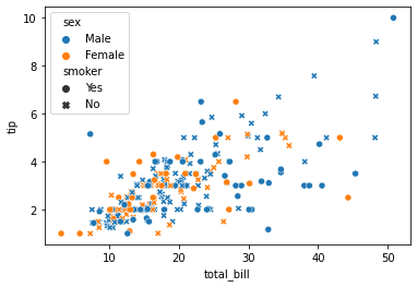
Numerical and categorical
If one variable is numeric and the other is categorical, there are several graphs that we can use for bivariate and multivariate analysis.
1) Bar graphic
The bar chart is a simple diagram that we can use to plot a categorical variable on the x-axis and a numeric variable on the y-axis and explore the relationship between both variables.. The black tip at the top of each bar shows the confidence interval. Let's explore P-Class with age.
sns.barplot(data['Pclass'], data['Age'])
plt.show()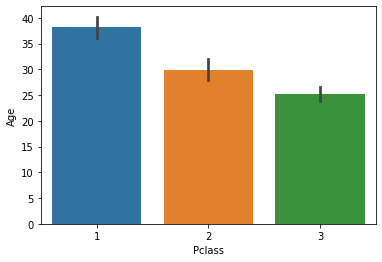
Multivariate analysis through bar graph
Hue's argument is very useful and helps to analyze more than 2 variables. Now, along with the above linking, we want to do with gender.
sns.barplot(data['Pclass'], data['Fare'], hue = data["Sex"])
plt.show()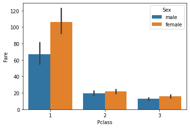
2) Box plot
We have already studied about box plotsBox Diagrams, Also known as box and whisker diagrams, are statistical tools that represent the distribution of a dataset. These diagrams show the median, quartiles and outliers, allowing data variability and symmetry to be visualized. They are useful in comparison between different groups and in exploratory analysis, making it easier to identify trends and patterns in the data.... in the previous univariate analysis. we can draw a separate box plot for both variables. Let's explore gender with age using a box plot.
sns.boxplot(data['Sex'], data["Age"])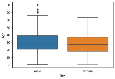
Multivariate analysis with box plot
Along with age and gender, let's see who has survived and who has not.
sns.boxplot(data['Sex'], data["Age"], data["Survived"])
plt.show()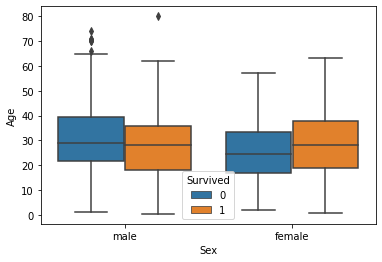
3) Distplot
Distplot explains PDF function through kernel density estimation. Distplot does not have a pitch parameter, but we can create it. Suppose we want to see the probability of people with a survival probability age range and find out whose survival probability is high for the mortality rate age range.
sns.distplot(data[data['Survived'] == 0]['Age'], hist=False, color="blue")
sns.distplot(data[data['Survived'] == 1]['Age'], hist=False, color="orange")
plt.show()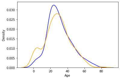
As we can see, the graphic is really very interesting. blue shows probability of dying and orange graph shows probability of survival. If we observe it, we can see that the probability of survival of children is greater than death and that it is the opposite in the case of the elderly. This little analysis sometimes says some important things about the data and helps when preparing data stories.
Categorical and categorical
Now we will work on categorical and categorical columns.
1) Heat mapa "heat map" is a graphical representation that uses colors to show the density of data in a specific area. Commonly used in data analytics, Marketing and behavioral studies, This type of visualization allows you to identify patterns and trends quickly. Through chromatic variations, Heat maps make it easier to interpret large volumes of information, helping to make informed decisions....
If you've ever used a pandas crosstab function, Heatmap is an equivalent visual representation of that only. Simply, shows how much presence of a category in link with another category is present in the data set. let me show first with the crosstab and later with the heatmap.
pd.crosstab(data['Pclass'], data['Survived'])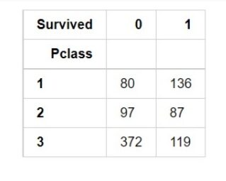
Now, with the heat map, we have to find how many people survived and died.
sns.heatmap(pd.crosstab(data['Pclass'], data['Survived']))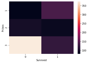
2) Cluster Map
we can also use a cluster map to understand the link between two categorical variables. A cluster map simply draws a dendrogram showing the categories of equivalent behavior together..
sns.clustermap(pd.crosstab(data['Parch'], data['Survived']))
plt.show()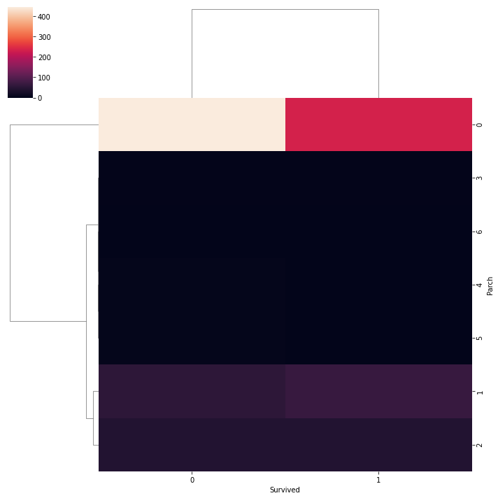
If you know clustering algorithms mainly on DBSCAN, then you should know the dendrogram. Then, these are all charts that are used primarily when doing exploratory analysis. There are a few more plots that you can draw as a violent plot, line pattern, a joint weft that are not primarily used.
The complete Notebook for more practice in EDA and data visualization is enabled in my Notebooks by kaggle, access it from here.
Final notes
EDA is just one key to understanding and representing your data in a better way, what, due, helps you build a powerful and more generalized model. Data visualization is easy to perform EDA, making it easier for others to understand our analysis.
I hope it was easy to catch up with all the plots that we have drawn. If you have any doubts, mention it in the comment section below. I will be happy to help you.
About the Author
Raghav Agrawal
I am pursuing my degree in computer science. I really like data science and big data. I love working with data and learning new technologies. Please, feel free to connect with me on Linkedin.





