
Overview
- Step-by-step approach to performing EDA
- Resources like blogs, MOOCS to become familiar with EDA
- Become familiar with various data visualization techniques, charts and diagrams.
- Demonstration of some steps with the Python code snippet
What differentiates one data science professional from another??
It's not machine learning, It is not deep learningDeep learning, A subdiscipline of artificial intelligence, relies on artificial neural networks to analyze and process large volumes of data. This technique allows machines to learn patterns and perform complex tasks, such as speech recognition and computer vision. Its ability to continuously improve as more data is provided to it makes it a key tool in various industries, from health..., it's not sql, is exploratory data analysis (EDA). How good is one with pattern identification? / hidden trends in the data and how valuable the insights are, is what sets data professionals apart.
1. What is exploratory data analysis?
Exploratory data analysis is an approach to analyze data sets to summarize their main features, often using statistical graphs and other data visualization methods.
EDA helps data science professionals in several ways: –
1 Get a better understanding of the data
2 Identify various data patterns
3 Better understand the problem statement
[ Note: the dataseta "dataset" or dataset is a structured collection of information, which can be used for statistical analysis, Machine learning or research. Datasets can include numerical variables, categorical or textual, and their quality is crucial for reliable results. Its use extends to various disciplines, such as medicine, economics and social science, facilitating informed decision-making and the development of predictive models.... in this blog is being opted as iris dataset]
2. Checking the introductory details about the data
The first and most important step of any data analysis, after uploading the data file, should consist of checking some introductory details. What, no. of columns, no. of rows, feature types (categorical or numerical), column entry data types.
Python code snippet
data.info ()
RangeIndex: 150 tickets, 0 a 149
data columns (5 columns in total):
# Non-Null Count Type Column
– —— ————– —–
0 sepal_length 150 not null float64
1 sepal_width 150 float64 not null
2 petal_length 150 not null float64
3 petal_width 150 not null float64
4 species 150 non null object
dtypes: float64 (4), object (1)
memory usage: 6.0+ KB
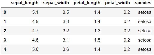
data.head () To display the first five rows
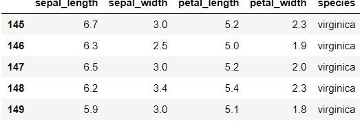
data.tail () to display the last five rows
3. statistical perspective
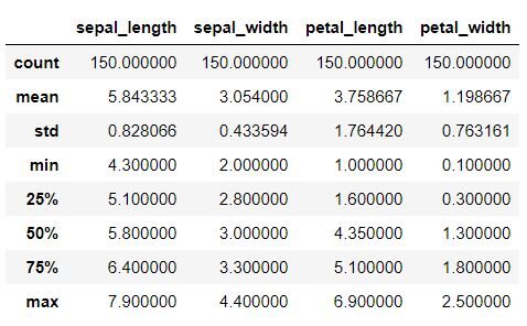
This step should be done to get details on various statistical data such as mean, standard deviation, medianThe median is a statistical measure that represents the central value of a set of ordered data. To calculate it, the data is organized from lowest to highest and the number in the middle is identified. If there are an even number of observations, the two core values are averaged. This indicator is especially useful in asymmetric distributions, since it is not affected by extreme values...., maximum value, minimum value.
Python code snippet
data.describe ()
4. Data cleansing
This is the most important step in EDA that involves removing rows / duplicate columns, fill empty entries with values as the mean / data median, remove multiple values, remove null entries
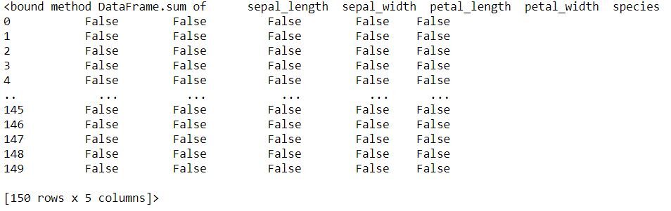
Null input check
Python code snippet
data.IsNull (). sum da el número de valores perdidos para cada variableIn statistics and mathematics, a "variable" is a symbol that represents a value that can change or vary. There are different types of variables, and qualitative, that describe non-numerical characteristics, and quantitative, representing numerical quantities. Variables are fundamental in experiments and studies, since they allow the analysis of relationships and patterns between different elements, facilitating the understanding of complex phenomena....
Remove null entries
Python code snippet
data.dropna (axis = 0, inplace = True) If there are null entries
Fill values instead of null inputs (if it is a numeric function)
Values can be mean, the median or any integer
Python code snippet
data[“sepal_length”].fillna (value = data[“sepal_length”].mean (), inplace = True) if there is a null input
Duplicate Check
Python code snippet
data.duplicated (). sum () returns the total number of duplicate entries
Remove duplicates
Python code snippet
data.drop_duplicates (inplace = True)
5. Data visualization
Data visualization is the method of converting raw data into a visual form., like a map or graph, to make the data easier to understand and extract useful information..
The main goal of data visualization is to put large data sets into a visual representation.. It is one of the important and easy steps when it comes to data science.
You can refer to the blog below for more details on data visualization.
Various types of visualization analysis are:
a. Univariate analysis:
This shows each observation / distribution of data on a single data variable.. Se puede mostrar con la ayuda de varios diagramas como Dispersion diagramThe scatter plot is a graphical tool used in statistics to visualize the relationship between two variables. It consists of a set of points in a Cartesian plane, where each point represents a pair of values corresponding to the variables analyzed. This type of chart allows you to identify patterns, Trends and possible correlations, facilitating data interpretation and decision-making based on the visual information presented...., line diagram, histogram plot (abstract), box plotsBox Diagrams, Also known as box and whisker diagrams, are statistical tools that represent the distribution of a dataset. These diagrams show the median, quartiles and outliers, allowing data variability and symmetry to be visualized. They are useful in comparison between different groups and in exploratory analysis, making it easier to identify trends and patterns in the data...., fiddle diagramThe violin diagram is a graphical representation that combines features of a boxplot and a density graph. Used to visualize the distribution of a dataset, showing both the median and variability through their shape, that resembles a violin. This type of graph is very useful in statistical analysis, ya que permite comparar múltiples distribuciones de forma clara y efectiva...., etc.
B. Bivariate analysis:
Bivariate analysis screens are performed to reveal the relationship between two data variables. It can also be shown with the help of scatter plots, histogramasHistograms are graphical representations that show the distribution of a dataset. They are constructed by dividing the range of values into intervals, O "Bins", and counting how much data falls in each interval. This visualization allows you to identify patterns, trends and variability of data effectively, facilitating statistical analysis and informed decision-making in various disciplines...., heat maps, box plots, violin diagrams, etc.
C. Analisis multivariable:
Multivariate analysis, as the name suggests, are displayed to reveal the relationship between more than two data variables.
Scatter diagrams, histogramas, box plots, fiddle plots can be used for multivariate analysis
several plots
Below are some of the charts that can be implemented for univariate analysis, bivariate and multivariate
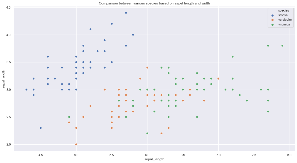
a. Scatter plotA scatter plot is a visual representation that shows the relationship between two numerical variables using points on a Cartesian plane. Each axis represents a variable, and the location of each point indicates its value in relation to both. This type of chart is useful for identifying patterns, Correlations and trends in the data, facilitating the analysis and interpretation of quantitative relationships....
Python code snippet
plt.figure (figsize = (17,9))
plt.title (‘Comparison between various species according to the length and width of the sapel’)
sns.scatterplot (data[‘sepal_length’],data[‘sepal_width’], tone = data[‘species’], s = 50)
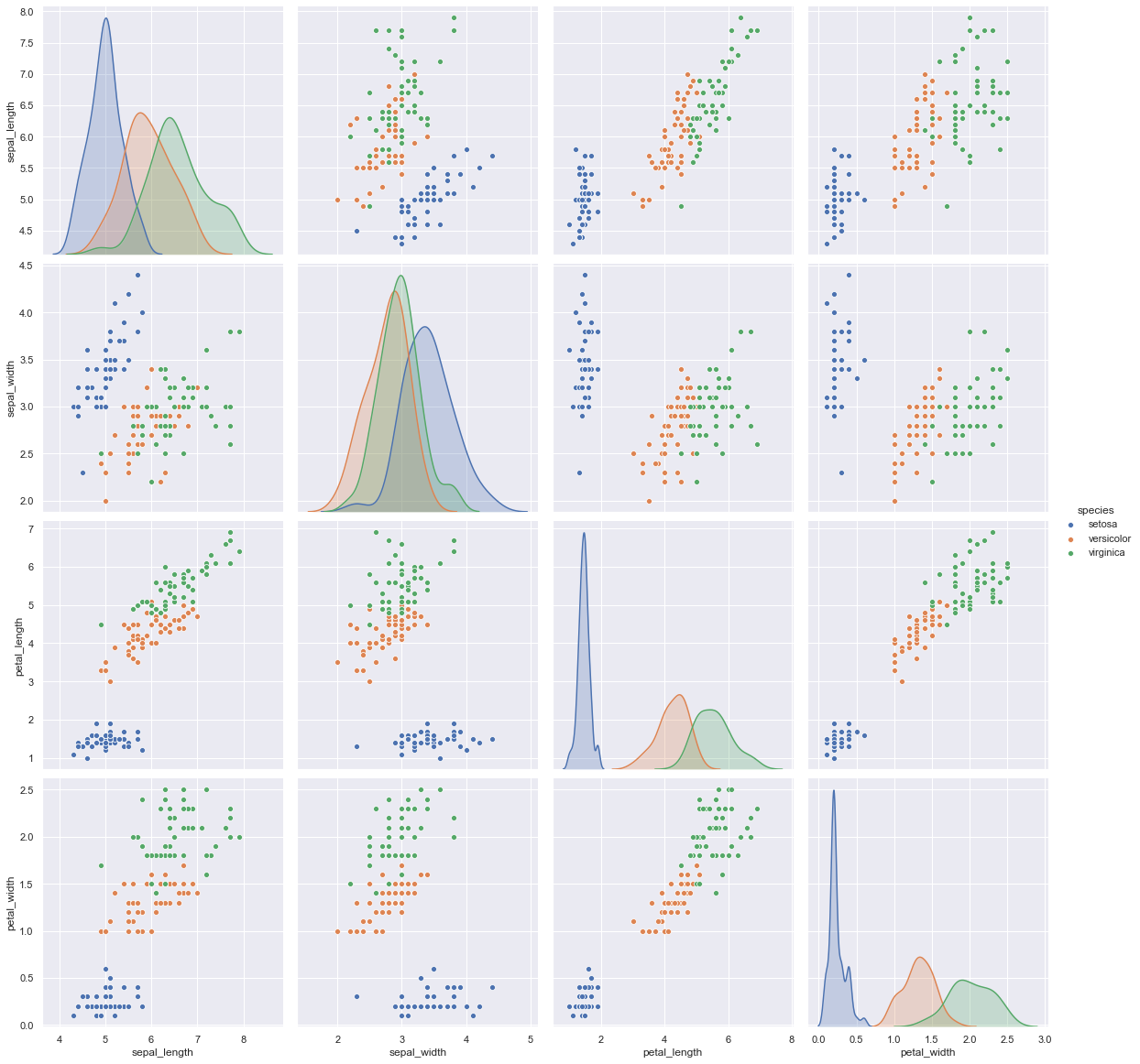
For multivariate analysis
Python code snippet
sns.pairplot (data, hue = ”species”, height = 4)
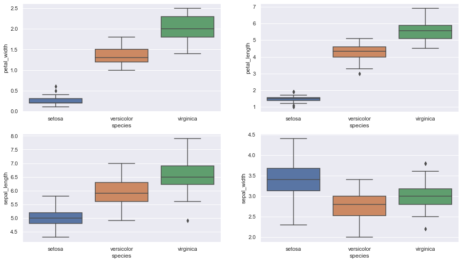
B. Box plot
Box plot to see how the categorical characteristic is distributed “Species” with the other four input variables
Python code snippet
fig, axes = plt.subplots (2, 2, figsize = (16,9))
sns.boxplot (y = “petal_width”, x = “species”, data = iris_data, orient = ‘v’, ax = axes[0, 0])
sns.boxplot (y = “petal_length”, x = “species”, data = iris_data, orient = ‘v’, ax = axes[0, 1])
sns.boxplot (y = ”sepal_length”, x = “species”, data = iris_data, orient = ‘v’, ax = axes[1, 0])
sns.boxplot (y = “sepal_width”, x = “species”, data = iris_data, orient = ‘v’, ax = ejes[1, 1])
plt.show ()
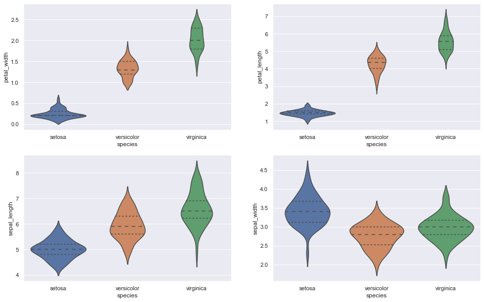
C. Violin frame
More informative than the box plot and shows the full distribution of the data.
Python code snippet
fig, axes = plt.subplots (2, 2, figsize = (16,10))
sns.violinplot (y = ”petal_width”, x = “species”, data = iris_data, orient = ‘v’, ax = axes[0, 0], inner = 'quartile')
sns.violinplot (y = “petal_length”, x = “species”, data = iris_data, orient = ‘v’, ax = ejes[0, 1], inner = 'quartile')
sns.violinplot (y = ”sepal_length”, x = “species”, data = iris_data, orient = ‘v’, ax = axes[1, 0], inner = 'quartile')
sns.violinplot (y = ”sepal_width”, x = “species”, data = iris_data, orient = ‘v’, ax = axes[1, 1], inner = 'quartile')
plt.show ()
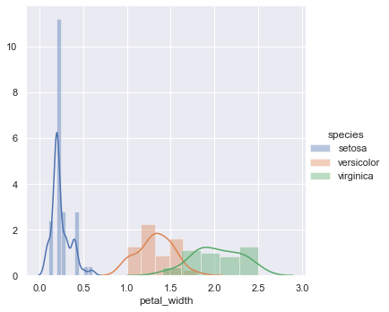
D. Histogramas
It can be used to visualize the probability density function (PDF)
Python code snippet
sns.FacetGrid (iris_data, hue = ”species”, height = 5)
.map (sns.distplot, “petal_width”)
.add_legend ();
With this I end this blog.
Hi everyone, Namaste
My name is Pranshu Sharma and i'm a data science enthusiast
Thank you very much for taking your valuable time to read this blog.. Feel free to point out any errors (after all, i am an apprentice) and provide the corresponding comments or leave a comment.
Dhanyvaad !!
Feedback:
Email: [email protected]
You can refer to the blog mentioned below to get familiar with exploratory data analysis.
The media shown in this article is not the property of DataPeaker and is used at the author's discretion.





