
This article was published as part of the Data Science Blogathon
draft. EDA is the process of investigating the data set to discover patterns and anomalies (Atypical values) and formulate hypotheses based on our understanding of the data set.
EDA involves generating summary statistics for numerical data in the dataset and creating various graphical representations to better understand the data.. In this article, we will understand EDA with the help of an example data set. we will use Piton idiom (Pandas library) for this purpose.

Libraries import
We will start by importing the libraries that we will need to perform EDA. These include NumPy, Pandas, Matplotlib y Seaborn.
import numpy as np
import pandas as pd
import matplotlib.pyplot as plt
%matplotlib inline
import seaborn as sns
Read data
Now we will read the data from a CSV file into a Pandas DataFrame. You can download the dataset for your reference.
df = pd.read_csv(r'C:UsersVipinData AnalyticsStudentsPerformance.csv')
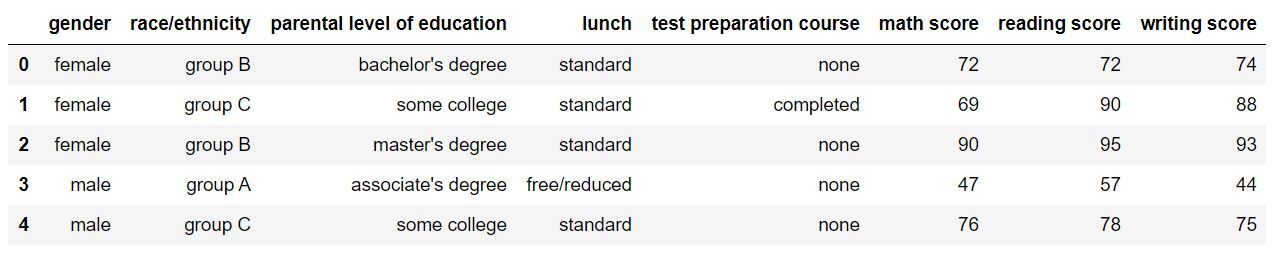
Let's take a look at what our dataset looks like using df.head (). The output should look like this:
Descriptive statistics
Perfect! Data looks exactly how we wanted. You can easily tell just by looking at the dataset that contains data about different students in a school / university and their scores in 3 subjects. Comencemos mirando los parametersThe "parameters" are variables or criteria that are used to define, measure or evaluate a phenomenon or system. In various fields such as statistics, Computer Science and Scientific Research, Parameters are critical to establishing norms and standards that guide data analysis and interpretation. Their proper selection and handling are crucial to obtain accurate and relevant results in any study or project.... estadísticos descriptivos para el conjunto de datos. We will use describe () for this.
df.describe(include="all")
By assigning the inclusion attribute a value of 'all', we make sure that categorical characteristics are also included in the result. The output DataFrame should look like this:
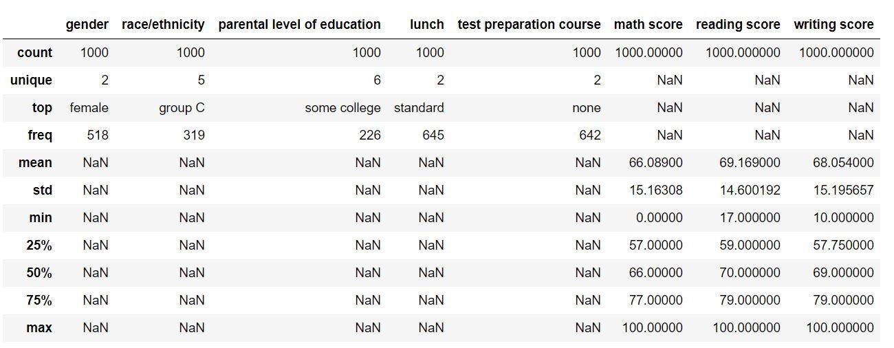
For numeric parameters, fields were filled as the mean, the standard deviation, percentiles and maximum. For categorical characteristics, the count has been completed, the only, the superior (most frequent value) and the corresponding frequency. This gives us a broad idea of our data set.
Missing value imputation
Now we will check for missing values. in our dataset. In case of missing tickets, we will impute them with the appropriate values (moda en caso de característica categórica y medianThe median is a statistical measure that represents the central value of a set of ordered data. To calculate it, the data is organized from lowest to highest and the number in the middle is identified. If there are an even number of observations, the two core values are averaged. This indicator is especially useful in asymmetric distributions, since it is not affected by extreme values.... o media en caso de característica numérica). We will use the isnull function () for this purpose.
df.isnull().sum()
This will tell us how many missing values we have in each column of our data set. The exit (Pandas Series) it should look like this:
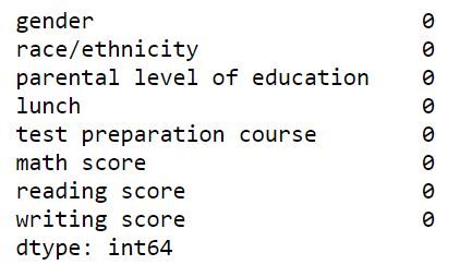
Fortunately for us, no missing values in this dataset. Now we will proceed to analyze this data set, observe patterns and identify outliers with the help of graphs and figures.
Graphic representation
We will start with Univariate analysis. We will use a bar graphicThe bar chart is a visual representation of data that uses rectangular bars to show comparisons between different categories. Each bar represents a value and its length is proportional to it. This type of chart is useful for visualizing and analyzing trends, facilitating the interpretation of quantitative information. It is widely used in various disciplines, such as statistics, Marketing and research, due to its simplicity and effectiveness.... for this purpose. We will observe the distribution of students by gender, race / ethnicity, their lunch status and whether they have an exam prep course or not.
plt.subplot(221)

df['gender'].value_counts().plot(kind='bar', title="Gender of students", figsize=(16,9))

plt.xticks(rotation=0)

plt.subplot(222)

df['race/ethnicity'].value_counts().plot(kind='bar', title="Race/ethnicity of students")

plt.xticks(rotation=0)

plt.subplot(223)

df['lunch'].value_counts().plot(kind='bar', title="Lunch status of students")

plt.xticks(rotation=0)

plt.subplot(224)

df['test preparation course'].value_counts().plot(kind='bar', title="Test preparation course")

plt.xticks(rotation=0)

plt.show()
The output should look like this:
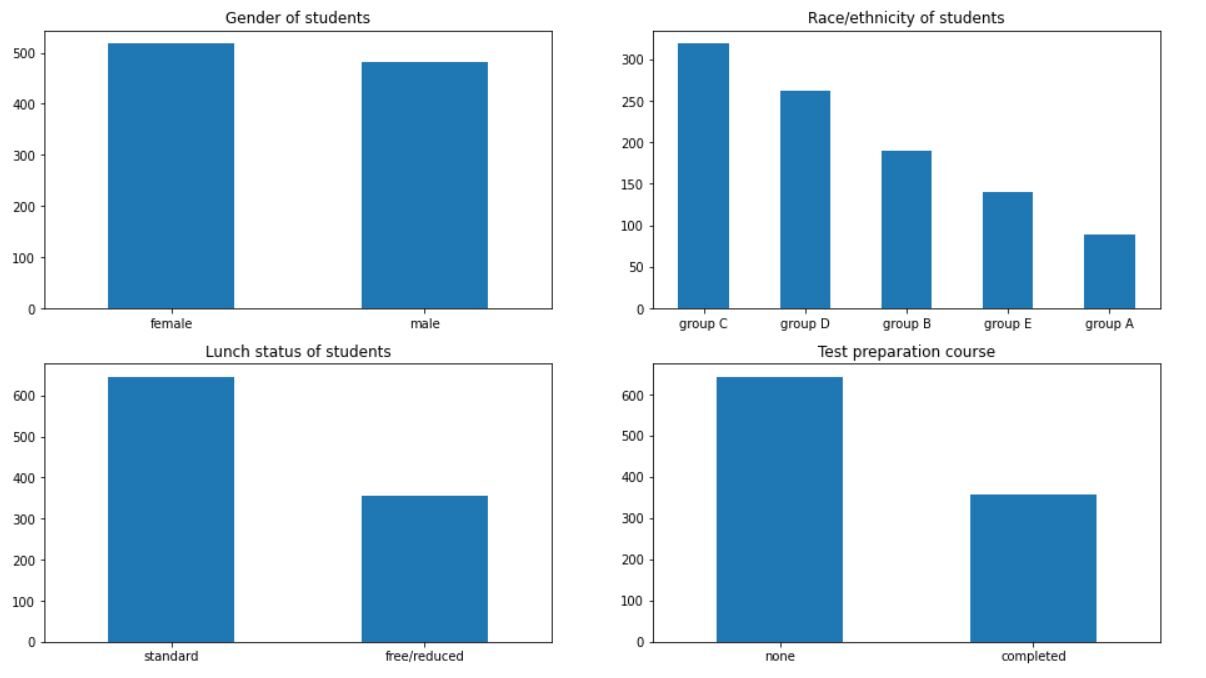
We can infer many things from the graph. There are more girls in school than boys. Most of the students belong to groups C and D. More than 60% of students have a standard lunch at school. What's more, more than 60% of students have not taken any exam preparation courses.
Continuing with the univariate analysis, then, we will do a box plot of the numeric columns (math score, reading score and writing score) in the data set. A box plot helps us visualize the data in terms of quartiles. Also identifies outliers in the data set, if there were. We will use the boxplot function () for this.
df.boxplot()
The output should look like this:
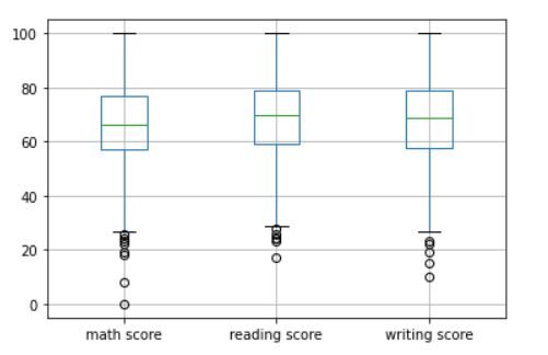
The middle portion represents the interquartile range (IQR). The horizontal green line in the middle represents the median of the data. Hollow circles near the tails represent outliers in the data set. But nevertheless, since it is quite possible for a student to score extremely low on a test, we will not eliminate these atypical values.
Now we will do a distribution plot of students' math scores. A distribution plot tells us how the data is distributed. We will use the distplot function.
sns.distplot(df['math score'])
The plot in the output should look like this:
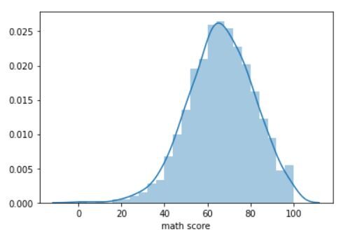
The graph represents a perfect bell curve up close. The peak is around 65 points, the mean of the students' math scores in the data set. A similar distribution plot can also be made for reading and writing scores..
Now we will see the correlation between 3 scores with the help of a heat mapa "heat map" is a graphical representation that uses colors to show the density of data in a specific area. Commonly used in data analytics, Marketing and behavioral studies, This type of visualization allows you to identify patterns and trends quickly. Through chromatic variations, Heat maps make it easier to interpret large volumes of information, helping to make informed decisions..... For this, we will use the corr function () y heatmap () for this exercise.
corr = df.corr()
sns.heatmap(corr, annot=True, square=True)
plt.yticks(rotation=0)
plt.show()
The plot in the output should look like this:
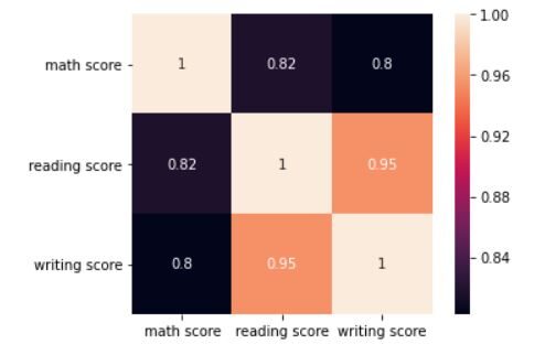
The heat map shows that 3 scores are highly correlated. The reading score has a correlation coefficient of 0,95 with writing score. The math score has a correlation coefficient of 0,82 with the reading score and 0,80 with writing score.
Now we will move on to Bivariate analysis. We will look at one relational plot en Seaborn. It helps us understand the relationship between 2 variables in different subsets of the data set. We will try to understand the relationship between the math score and the writing score of students of different genders.
sns.relplot(x='math score', y='writing score', hue="gender", data=df)
The relational plot should look like this:
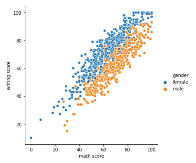
The graph shows a clear difference in scores between male and female students. For the same score in math, female students are more likely to have higher writing scores than male students. But nevertheless, for the same writing score, male students are expected to score higher in math than female students.
Relational graphs help us to perform bivariate analysis. You can refer to the documentation of the relplot function () en Seaborn here.
Finally, we will analyze the performance of students in mathematics, reading and writing according to the level of education of your parents and the course of preparation for the exam. First, Let's take a look at the impact of parents' education level on their children's performance in school using a line graph.
df.groupby('parental level of education')[['math score', 'reading score', 'writing score']].mean().T.plot(figsize=(12,8))
The output will look like this:
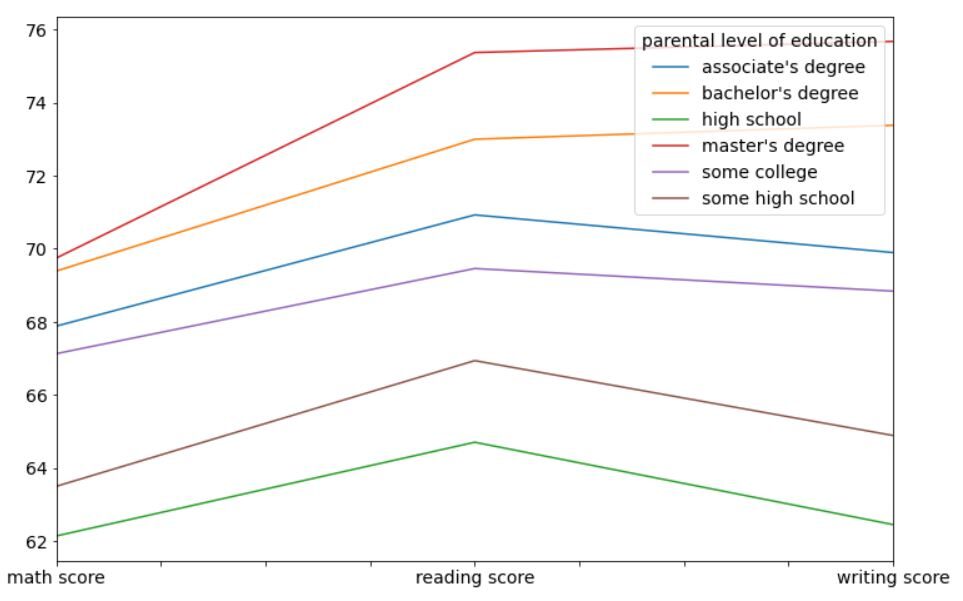
It is very clear from this graph that students whose parents are more educated than others (master's degree, bachelor's and associate's degree) perform better on average than students whose parents have less education (high school). This may be a genetic difference or simply a difference in the students' home environment. More educated parents are more likely to push their students toward studies.
Secondly, Let's look at the impact of the test preparation course on student performance using a horizontal bar chart.
df.groupby('test preparation course')[['math score', 'reading score', 'writing score']].mean().T.plot(kind='barh', figsize=(10,10))
The output should look like this:
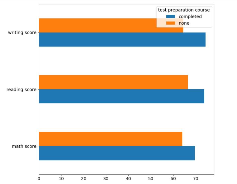
One more time, it is very clear that students who have completed the exam preparation course have performed better, on average, compared to students who have not opted for the course.
Final notes
In this article, we understood the meaning of Exploratory Data Analysis (EDA) with the help of a sample data set. We look at how we can analyze the data set, draw conclusions from it and form a hypothesis based on that.
The author of this article is Vishesh Arora. You can connect with me at LinkedIn.
The media shown in this article is not the property of DataPeaker and is used at the author's discretion.





