
This article was published as part of the Data Science Blogathon.
Introduction
Gradient Descent is one of the most widely used machine learning algorithms in the industry. Y, but nevertheless, confuses many newcomers.
I get it! The mathematics behind the increase of gradientGradient is a term used in various fields, such as mathematics and computer science, to describe a continuous variation of values. In mathematics, refers to the rate of change of a function, while in graphic design, Applies to color transition. This concept is essential to understand phenomena such as optimization in algorithms and visual representation of data, allowing a better interpretation and analysis in... is not easy if you are just starting. My goal is to help you get an insight behind gradient descent in this article..

We will quickly understand the role of a cost function, the gradient descent explanation, how to choose the learning parameter and the effect of overshooting on the gradient descent. Let's start!
What is a cost function?
It's a function which measures the performance of a model for any given data. Cost function quantifies the error between predicted and expected values and presents it as a single real number.
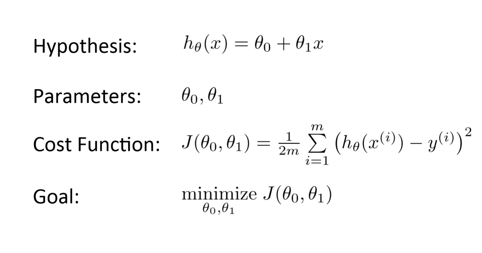
After making a hypothesis with parametersThe "parameters" are variables or criteria that are used to define, measure or evaluate a phenomenon or system. In various fields such as statistics, Computer Science and Scientific Research, Parameters are critical to establishing norms and standards that guide data analysis and interpretation. Their proper selection and handling are crucial to obtain accurate and relevant results in any study or project.... initials, we calculate the Cost function. And with the aim of reducing the cost function, we modify the parameters using the gradient descent algorithm on the given data. Here is the mathematical representation for it:
What is Gradient Descent?
The million dollar question!
Let's say you are playing a game where the players are on top of a mountain and are asked to reach the lowest point of the mountain.. What's more, they are blindfolded. Then, What approach do you think would get you to the lake?
Take a moment to think about this before reading on..
The best way is to observe the ground and find where the ground descends. From that position, step down and iterate through this process until you reach the lowest point.
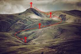 Finding the lowest point in a mountainous landscape. (Source: Fisseha Berhane)
Gradient descent is an Optimization algorithmAn optimization algorithm is a set of rules and procedures designed to find the best solution to a specific problem, maximizing or minimizing a target function. These algorithms are fundamental in various areas, such as engineering, The economy and artificial intelligence, where it seeks to improve efficiency and reduce costs. There are multiple approaches, including genetic algorithms, Linear programming and combinatorial optimization methods.... iterative method to find the local minimum of a function.
To find the local minimum of a function using gradient descent, we must take steps proportional to the negative of the gradient (move away from the gradient) of the function at the current point. If we take steps proportional to the positive of the gradient (moving towards the gradient), we will approach a local maximum of the function, and the procedure is called Gradient rise.
Gradient descent was originally proposed by CAUCHY in 1847. Also known as steepest descent.
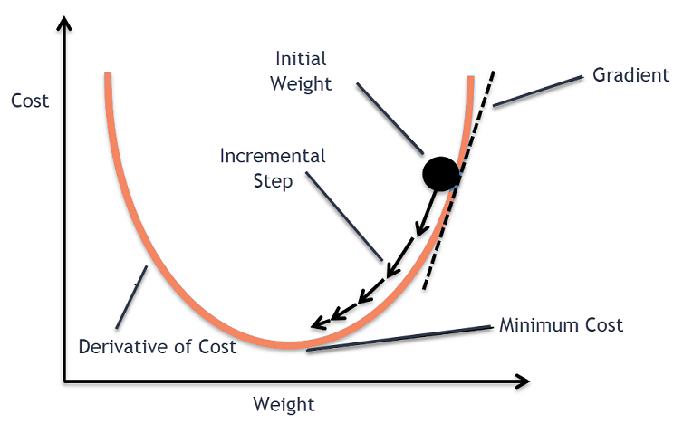
The goal of the gradient descent algorithm is to minimize the given function (for instance, cost function). To achieve this goal, performs the steps iteratively:
- Calculate the gradient (pending), the first-order derivative of the function at that point
- Take a step (move on) in the opposite direction of the gradient, the opposite direction of the slope increases from the current point in alpha times the gradient at that point
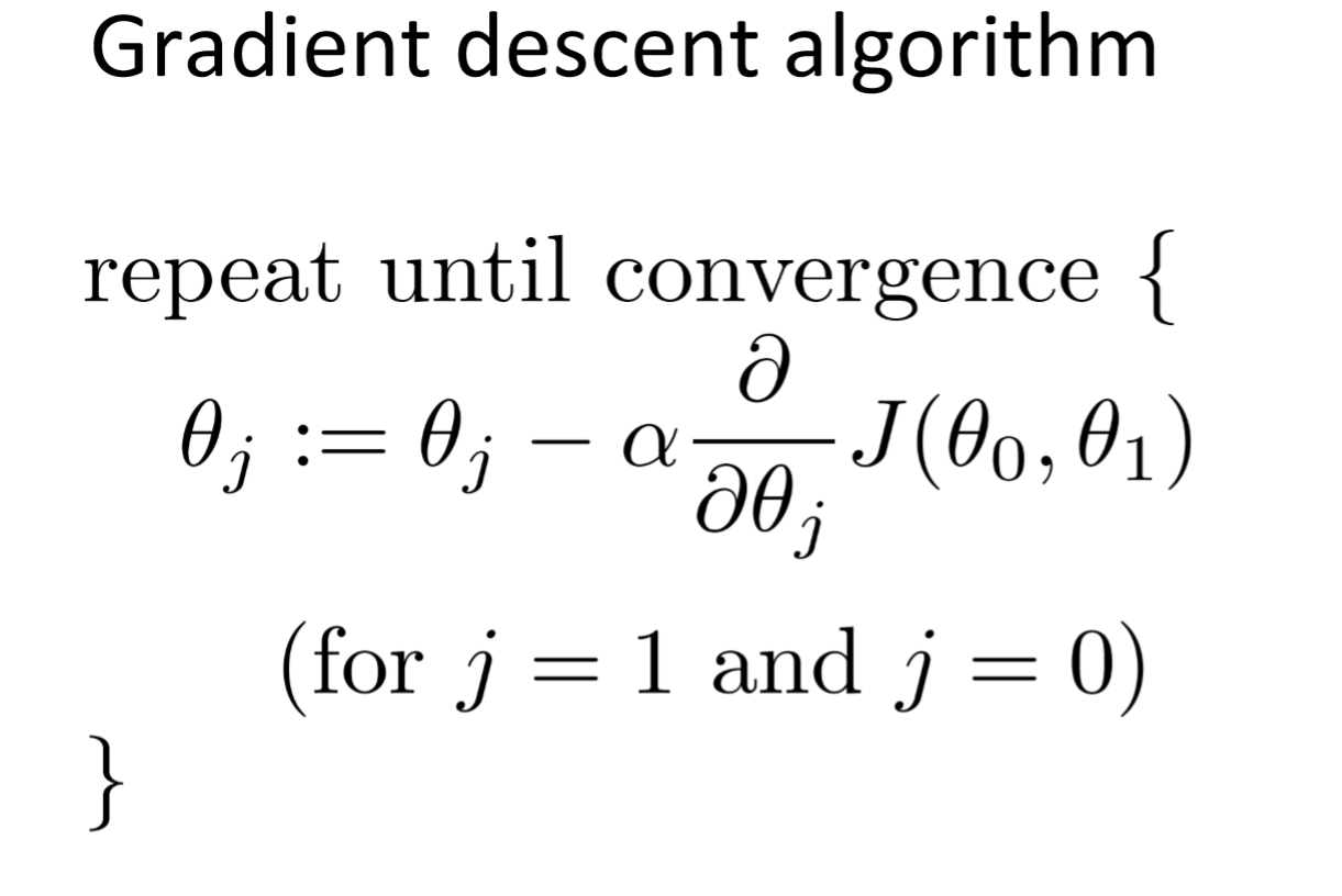
Alpha is called Learning rate – a tuning parameter in the optimization process. Decide on the length of the steps.
Plotting the gradient descent algorithm
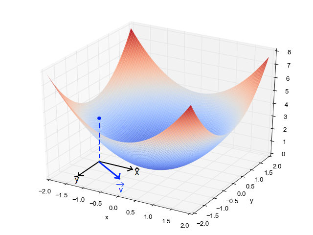
When we have only one parameter (theta), we can plot the cost of the variableIn statistics and mathematics, a "variable" is a symbol that represents a value that can change or vary. There are different types of variables, and qualitative, that describe non-numerical characteristics, and quantitative, representing numerical quantities. Variables are fundamental in experiments and studies, since they allow the analysis of relationships and patterns between different elements, facilitating the understanding of complex phenomena.... dependent variable on the y-axis and theta on the x-axis. If there are two parameters, we can opt for a 3-D graph, with the cost on one axis and the two parameters (thetas) along the other two axes.
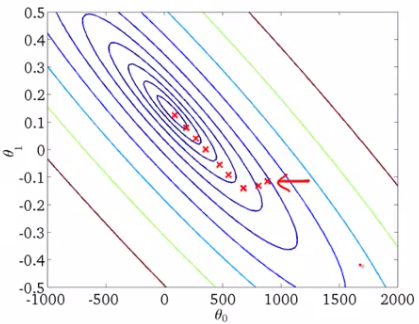
It can also be viewed using contours. This shows a 3D graph in two dimensions with parameters along both axes and the response as a contour. The value of the response increases away from the center and has the same value along with the rings. The answer is directly proportional to the distance from a point to the center (along one direction).
Alpha – The learning rate
We have the direction we want to move, now we must decide the size of the step we must take.
* Must be chosen carefully to end with local minimums.
- If the learning rate is too high, we could EXCEED the lows and keep bouncing, without reaching the minimum
- If the learning rate is too small, training may be too long.
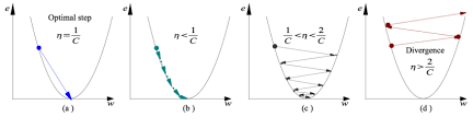
- a) The learning rate is optimal, the model converges to the minimum
- b) The learning rate is too small, takes longer but converges to a minimum
- c) The learning rate is greater than the optimal value, surpasses but converges (1 / C <the <2 / C)
- d) The learning rate is very large, it surpasses and diverges, moves away from the minimum, performance decreases in learning
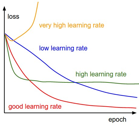
Note: As the gradient decreases while moving towards the local minima, step size decreases. Therefore, the learning rate (alfa) can be constant during optimization and no need to vary iteratively.
Local minima
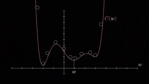
The cost function can consist of many minimum points. The gradient can settle at any of the minimums, which depends on the starting point (namely, the initial parameters (theta)) and the learning rate. Therefore, optimization can converge at different points with different starting points and learning rate.
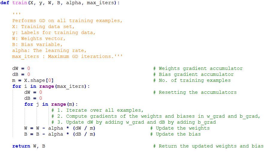
Implementing Gradient Descent Code in Python
Final notes
Once we tune the learning parameter (alfa) and we obtain the optimal learning rate, we begin to iterate until we converge to the local minima.





