This article was published as part of the Data Science Blogathon.
Introduction
In the previous post, we define the probability distributions and briefly discuss the different discrete probability distributions. In this post, we will continue to learn about probability distributions through continuous probability distributions.
Definition
If you remember our previous discussion, continuous random variables can take an infinite number of values in a given interval. For instance, in the interval [2, 3] there are infinite values between 2 Y 3. Continuous distributions are defined by the probability density functions (PDF) instead of probability mass functions. The probability that a continuous random variable equals an exact value is always zero. Continuous probabilities are defined over an interval. For instance, P (X = 3) = 0 but P (2.99 <X <3.01) can be calculated by integrating the PDF over the interval [2.99, 3.01]
List of continuous probability distributions
Then, we analyze the most used continuous probability distributions:
1. Continuous uniform distribution
The uniform distribution has both continuous and discrete shapes. Here, we discuss the continuum. This distribution plots the random variables whose values are equally likely to occur. The most common example is rolling a fair dice. Here, the 6 results are just as likely to occur. Therefore, the probability is constant.
Consider the example where a = 10 and b = 20, the layout looks like this:
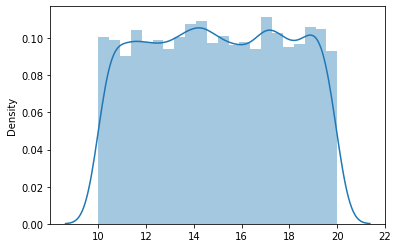
The PDF is given by,
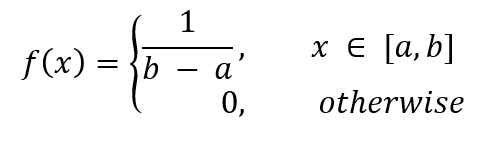
where a is the minimum value and b is the maximum value.
2. Normal distribution
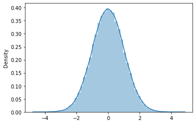
This is the most discussed and most frequently found distribution in the real world.. Many continuous distributions often achieve a normal distribution given a large enough sample. This has two parameters, namely, the standard deviation and the mean.
This distribution has many interesting properties. The mean has the highest probability and all other values are equally distributed on both sides of the mean symmetrically. The standard normal distribution is a special case where the mean is 0 and the standard deviation of 1.
It also follows the empirical formula that the 68% of the values are at 1 distance standard deviation, the 95% percent of them are 2 distance standard deviations and the 99,7% are to 3 standard deviations from the mean. This property is very useful when designing hypothesis tests (https://www.statisticshowto.com/probability-and-statistics/hypothesis-testing/).
The PDF is given by,
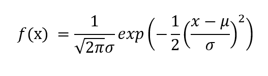
where μ is the mean of the random variable X and σ is the standard deviation.
3. Logarithmic normal distribution
This distribution is used to graph the random variables whose log values follow a normal distribution.. Consider the random variables X and Y. Y = ln (X) is the variable that is represented in this distribution, where ln denotes the natural logarithm of the values of X.
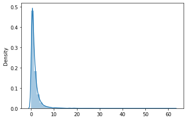
The PDF is given by,
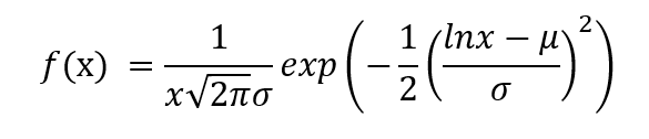
where μ is the mean of Y and σ is the standard deviation of Y.
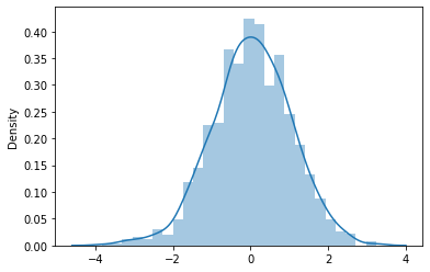
4. Student's t distribution
Student's t distribution is similar to the normal distribution. The difference is that the tails of the distribution are thicker. Used when the sample size is small and the population variance is unknown. This distribution is defined by the degrees of freedom (p) which are calculated as the sample size minus 1 (n – 1).
As the sample size increases, degrees of freedom increase, the t distribution approaches the normal distribution and the tails become narrower and the curve approaches the mean. This distribution is used to test estimates of the population mean when the sample size is less than 30 and the population variance is unknown. Variance / sample standard deviation is used to calculate the t-value.
The PDF is given by,
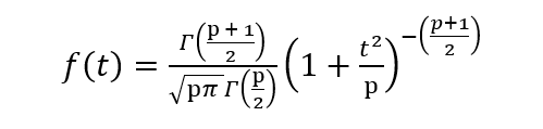
where p are the degrees of freedom and Γ is the gamma function. See this link for a short description of the gamma function.
The t statistic used in the hypothesis test is calculated as follows,
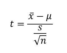
where x̄ is the sample mean, μ the population mean and s is the sample variance.
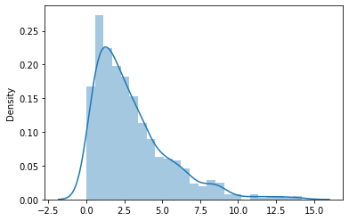
5. Chi-square distribution
This distribution is equal to the sum of squares of p normal random variables. p is the number of degrees of freedom. Like the t distribution, as degrees of freedom increase, the distribution gradually approaches the normal distribution. Below is a chi-square distribution with three degrees of freedom.
The PDF is given by,
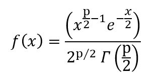
where p are the degrees of freedom and Γ is the gamma function.
The chi-square value is calculated as follows:
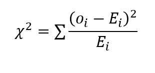
where o is the observed value and E represents the expected value. This is used in hypothesis testing to draw inferences about the population variance of the normal distributions..
6. Exponential distribution
Remember the discrete probability distribution that we discussed in the Discrete Probability post. In the Poisson distribution, we take the example of calls received by the customer service center. In that example, we consider the average number of calls per hour. Now, in this distribution, the time between successive calls is explained.
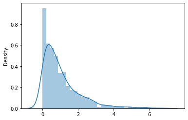
The exponential distribution can be viewed as an inverse of the Poisson distribution. The events under consideration are independent of each other.
The PDF is given by,
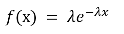
where λ is the rate parameter. λ = 1 / (mean time between events).
To complete, we have very briefly discussed different continuous probability distributions in this post. Feel free to add comments or suggestions below.
About me
Soy Priyanka Madiraju, a former software engineer working on the transition to data science. I am a Master's student in Data Science. Feel free to connect with me at https://www.linkedin.com/in/priyanka-madiraju
The media shown in this article is not the property of DataPeaker and is used at the author's discretion.


