
This post was released as part of the Data Science Blogathon.
Do you find AI and ML interesting??
Are you interested in becoming a machine learning engineer?? Have you learned programming languages like Python or R, but has difficulty moving forward? (This happens mainly in the case of self-taught). Do you find words like Statistics intimidating?, Probability and Regression? It's absolutely understandable to feel like this, especially if you come from a non-technical background. But there is a solution for this. And it is …. to start. Remember, if it never starts, you will never make mistakes and you may never learn. So start small.
Simple linear regression
When do we use LR?
We are going to create a simple machine learning model using linear regression. But before moving on to the coding part, let's look at the basics and the logic behind it. Regression is used in the supervised machine learning algorithm, which is the most used algorithm at the moment. El análisis de regresión es un método en el que establecemos una vinculación entre una variableIn statistics and mathematics, a "variable" is a symbol that represents a value that can change or vary. There are different types of variables, and qualitative, that describe non-numerical characteristics, and quantitative, representing numerical quantities. Variables are fundamental in experiments and studies, since they allow the analysis of relationships and patterns between different elements, facilitating the understanding of complex phenomena.... dependent (Y) and an independent variable (x); which enables us to predict and forecast the results. Do you remember solving equations like y = mx + c of your school days? If so, Congratulations. You already know simple linear regression. If that is not the case, not difficult to learn at all.
Let's consider a popular example. The number of hours invested in the study and the marks obtained in the exam. In this circumstance, the grades obtained depend on the number of hours the student invests in studying, therefore, the grades obtained are the dependent variable y and the number of hours is the independent variable x. The objective is to develop a model that helps us predict the grades obtained for a new number of hours.. We are going to achieve it using Linear Regression.
To be very clear about this concept, let's consider another example. In a data set with the amount of calories consumed and the weight gained, the weight gained depends on the calories consumed by a person. Therefore, the weight gained is the dependent variable y and the number of calories is the independent variable x.
y = mx + c is the equation of the regression line that best fits the data and, sometimes, furthermore it is represented as y = b0 + b1X. Here,
y is the dependent variable, in this circumstance, the grades obtained.
x is the independent variable, in this circumstance, the number of hours.
mo b1 is the slope of the regression line and the coefficient of the independent variable.
c o b0 is the intersection of the regression line.
The logic is to calculate the slope (m) and intercept (c) with the available data and then we will be able to calculate the value of y for any value of x.
Python packages and codes required
Now, How to perform linear regression in python? We need to import some packages, namely NumPy to work with matrices, Sklearn to perform linear regression, Y Matplotlib to plot the regression line and graphs. Note that it is almost impossible to have knowledge of every package and library in Python, especially for beginners. Therefore, it is recommended to keep looking for the right package when needed for a task. It's easier to remember to use packages with hands-on experience involved, instead of just theoretically reading the documentation available on them.
Moving on to the coding part. The first step is to import the required packages.
import numpy as np
import matplotlib.pyplot as plt
from sklearn.linear_model import LinearRegression
Considering this is your first machine learning model, we will eliminate some complications by taking a very small sample, en lugar de utilizar datos de una databaseA database is an organized set of information that allows you to store, Manage and retrieve data efficiently. Used in various applications, from enterprise systems to online platforms, Databases can be relational or non-relational. Proper design is critical to optimizing performance and ensuring information integrity, thus facilitating informed decision-making in different contexts.... great. This will also help to clearly see the result in the graphics and to appreciate the concept effectively..
xpuntos = np.array ([10, 11, 12, 13, 14, 15]) .reform (-1,1)
ypoints = np.array ([53, 52, 60, 63, 72, 70])
Notice that we are remodeling the xpoints have one column and many rows. The predictor (x) must be an array of arrays and the solution (Y) can be a simple matrix.
A variable Linreg is created as an instance of Linear regression. It can take parameters that are optional. They are not needed for this example, so we will ignore them. As the name suggests, the .to fit in() The method fits the model and is used to estimate some of the model parameters, which means it calculates the optimized value of myc using the given data.
linreg = LinearRegression()
linreg.fit(xpoints, ypoints)
.predict() The method is used to obtain the predicted solution using the model and takes the predictor xpoints as an argument.
y_pred = linreg.predict(xpoints)
Now, print y_pred and notice that the values are quite close to points. If the predicted and actual responses have a value close to, means the model is accurate. In an ideal case, the predicted and actual response values would overlap.
The pyplot module from the Matplotlib library has been imported as plt. Then we can easily plot the graphs using .dispersion() which takes xpoints Y points as arguments. Plot the real solution. The predicted solution is plotted using.plot() function. The chart can be labeled using.xlabel Y .ylabel.
plt.scatter (x points, points and)
plt.plot (x points, y_pred)
plt.xlabel (“x points”)
plt.ylabel (“points and”)
plt.show ()
plt.show () muestra todos los objetos de figure"Figure" is a term that is used in various contexts, From art to anatomy. In the artistic field, refers to the representation of human or animal forms in sculptures and paintings. In anatomy, designates the shape and structure of the body. What's more, in mathematics, "figure" it is related to geometric shapes. Its versatility makes it a fundamental concept in multiple disciplines.... en este momento activos.
Attributes .coef_ Y .intercept_ gives the slope which is also the coefficient of x, and the intersection of y. It means that y = c = 8.80, about, when x = 0 and y = 4.22 (1) + 8.80 = 13.02 (about) when x = 1. Note that in the output the intersection is scalar and the coefficient is a matrix.
print(linreg.coef_)
print(linreg.intercept_)
We have built our model. Now try to predict the solution y_new for a new predictor value x_new = 16. There! We have a model that can predict the solution for any given predictor.
x_new = np.array ([16]) .reform (-1,1)
y_new = linreg.predict (x_new)
to print (y_new)
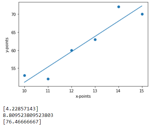
The image above is what the final result might look like. The 3 outputs below the graph are the solution to our Print() statements. Then they are pending, intersection and y_new respectively.
The equation of the regression line is y = 4.23x + 8,80. Then, according to the equation, when x = 16,
y = 4,23 * (16) + 8,80 = 76,48. The small difference in the calculation is due to the decimal points.
We can use .score() method that samples x and y as their 2 arguments to find R2 or the coefficient of determination. Best value for R2 it is 1.0 and it can also take negative values, since the model may be worse. A closer value of R2 a 1.0 indicates the efficiency of our model.
linreg.score(xpoints, ypoints)
Run the code and you will see that the value of R2 it is 0,89, so the model forecast is reliable.
Whats Next?
This is as simple as a linear regression. It's not the only way, but it seemed to me the simplest and easiest way. Don't stop here. When you feel comfortable with this, you can go one step further and consider a larger data set. As an example, a CSV file. You will need to work with Pandas and NumPy packages in that case. Then, you can test a linear or multiple logistic regression model. Keep learning and practicing.
The media shown in this post is not the property of DataPeaker and is used at the author's discretion.





