This article was published as part of the Data Science Blogathon
Los diversos métodos de deep learningDeep learning, A subdiscipline of artificial intelligence, relies on artificial neural networks to analyze and process large volumes of data. This technique allows machines to learn patterns and perform complex tasks, such as speech recognition and computer vision. Its ability to continuously improve as more data is provided to it makes it a key tool in various industries, from health... utilizan datos para entrenar algoritmos de redes neuronales para realizar una variedad de tareas de aprendizaje automático, as the classification of different classes of objects. Convolutional neural networks are very powerful deep learning algorithms for image analysis. This article will explain how to build, train and evaluate convolutional neural networks.
You will also learn how to improve your ability to learn from data and how to interpret training results.. Deep Learning has several applications such as image processing, natural language processing, etc. It is also used in Medical Sciences, Media and Entertainment, Autonomous Cars, etc.
What is CNN?
CNN is a powerful algorithm for image processing. These algorithms are currently the best algorithms we have for automated image processing.. Many companies use these algorithms to do things like identify objects in an image.
Images contain RGB combination data. Matplotlib can be used to import an image into memory from a file. The computer does not see an image, all you see is an array of numbers. Color images are stored in three-dimensional arrays. The first two dimensions correspond to the height and width of the image (the number of pixels). La última dimension"Dimension" It is a term that is used in various disciplines, such as physics, Mathematics and philosophy. It refers to the extent to which an object or phenomenon can be analyzed or described. In physics, for instance, there is talk of spatial and temporal dimensions, while in mathematics it can refer to the number of coordinates necessary to represent a space. Understanding it is fundamental to the study and... corresponde a los colores rojo, green and blue present in every pixel.
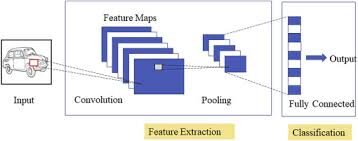
Three layers of CNN
Specialized convolutional neural networks for image and video recognition applications. CNN is mainly used in image analysis tasks such as image recognition, detección de objetos y segmentationSegmentation is a key marketing technique that involves dividing a broad market into smaller, more homogeneous groups. This practice allows companies to adapt their strategies and messages to the specific characteristics of each segment, thus improving the effectiveness of your campaigns. Targeting can be based on demographic criteria, psychographic, geographic or behavioral, facilitating more relevant and personalized communication with the target audience.....
There are three types of layers in convolutional neural networks:
1) convolutional coverThe Convolutional Layer, fundamental in convolutional neural networks (CNN), It is mainly used for data processing with grid-like structures, as pictures. This layer applies filters that extract relevant features, such as edges and textures, allowing the model to recognize complex patterns. Its ability to reduce the dimensionality of data and maintain essential information makes it a key tool in computer vision tasks..: in a red neuronalNeural networks are computational models inspired by the functioning of the human brain. They use structures known as artificial neurons to process and learn from data. These networks are fundamental in the field of artificial intelligence, enabling significant advancements in tasks such as image recognition, Natural Language Processing and Time Series Prediction, among others. Their ability to learn complex patterns makes them powerful tools.. típica, each input neuron is connected to the next hidden layer. And CNN, solo una pequeña región de las neuronas de la input layerThe "input layer" refers to the initial level in a data analysis process or in neural network architectures. Its main function is to receive and process raw information before it is transformed by subsequent layers. In the context of machine learning, Proper configuration of the input layer is crucial to ensure the effectiveness of the model and optimize its performance in specific tasks.... se conecta a la capa oculta de neuronas.
2) Grouping layer: the grouping layer is used to reduce the dimensionality of the feature map. There will be multiple layers of activation and grouping within the hidden layer of CNN.
3) Fully connected layer: Fully connected layers form the last covers In the net. The entrance to the fully connected layer is the output of the final grouping or convolution Front cover, which is flattened and then introduced into the fully connected layer.
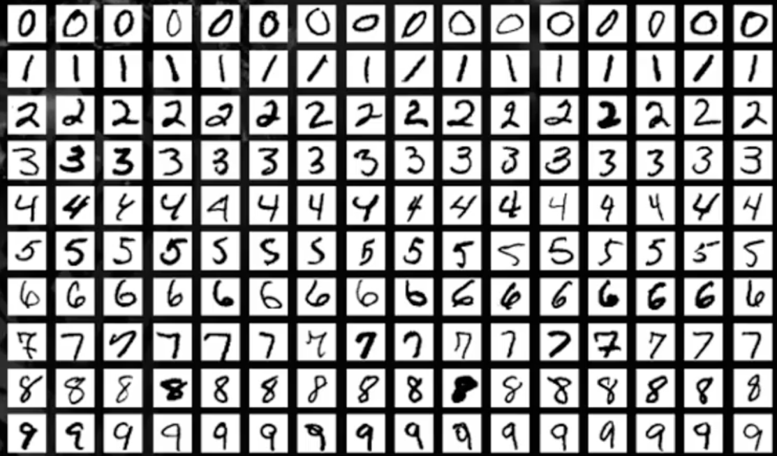
MNIST data set
In this article, we will work on object recognition in image data using the MNIST data set for handwritten digit recognition.
The MNIST dataset consists of digit images from a variety of scanned documents. Each image is a square of 28 x 28 pixels. In this data set, are used 60.000 images to train the model and 10.000 pictures to test the model. There is 10 digits (0 a 9) O 10 classes to predict.
Loading the MNIST dataset
Instale la biblioteca de TensorFlow e importe el conjunto de datos como un conjunto de datos de trainingTraining is a systematic process designed to improve skills, physical knowledge or abilities. It is applied in various areas, like sport, Education and professional development. An effective training program includes goal planning, regular practice and evaluation of progress. Adaptation to individual needs and motivation are key factors in achieving successful and sustainable results in any discipline.... and test.
Plot the image sample output
!pip install tensorflow
from keras.datasets import mnist
import matplotlib.pyplot as plt
(X_train,y_train), (X_test, y_test)= mnist.load_data()
plt.subplot()
plt.imshow(X_train[9], cmap=plt.get_cmap('gray'))
Production:

Deep learning model with multilayer perceptrons using MNIST
In this model, we will create a simple neural network model with a single hidden layer for the MNIST dataset for handwritten digit recognition.
A perceptron is a single neuron model that is the building block of the largest neural networks. The multilayer perceptron consists of three layers, namely, the input layer, the hidden layer and the Output layerThe "Output layer" is a concept used in the field of information technology and systems design. It refers to the last layer of a software model or architecture that is responsible for presenting the results to the end user. This layer is crucial for the user experience, since it allows direct interaction with the system and the visualization of processed data..... The hidden layer is not visible to the outside world. Only the input layer and the output layer are visible. For all DL models, data must be numerical in nature.
Paso 1: import key libraries
import numpy as np
from keras.models import Sequential
from keras.layers import Dense
from keras.utils import np_utils
Paso 2: reshape the data
Each image is 28X28 in size, so there is 784 pixels. Then, the output layer has 10 Departures, the hidden layer has 784 neurons and the input layer has 784 tickets. Later, the dataset is converted to a float data type.
number_pix=X_train.shape[1]*X_train.shape[2]
X_train=X_train.reshape(X_train.shape[0], number_pix).astype('float32')
X_test=X_test.reshape(X_test.shape[0], number_pix).astype('float32')
Paso 3: normalize data
NN models generally require scaled data. In this code snippet, data is normalized from (0-255) a (0-1) and the variableIn statistics and mathematics, a "variable" is a symbol that represents a value that can change or vary. There are different types of variables, and qualitative, that describe non-numerical characteristics, and quantitative, representing numerical quantities. Variables are fundamental in experiments and studies, since they allow the analysis of relationships and patterns between different elements, facilitating the understanding of complex phenomena.... de destino se codifica en un solo uso para su posterior análisis. The target variable has a total of 10 lessons (0-9)
X_train=X_train/255
X_test=X_test/255
y_train= np_utils.to_categorical(y_train)
y_test= np_utils.to_categorical(y_test)
num_classes=y_train.shape[1]
print(num_classes)
Production:
10
Now, we will create a function NN_model and compile it
Paso 4: define model function
def nn_model():
    model=Sequential()
    model.add(Dense(number_pix, input_dim=number_pix, activation = 'reread'))
    mode.add(Dense(num_classes, activation='softmax'))
    model.compile(loss="categorical_crossentropy", optimize ="Adam", metrics=['accuracy'])
    return model
There are two layers, una es una capa oculta con la función de activación ReLuThe ReLU activation function (Rectified Linear Unit) It is widely used in neural networks due to its simplicity and effectiveness. is defined as ( f(x) = max(0, x) ), meaning that it produces an output of zero for negative values and a linear increment for positive values. Its ability to mitigate the problem of gradient fading makes it a preferred choice in deep architectures.... y la otra es la capa de salida que usa la función softmaxThe softmax function is a mathematical tool used in the field of machine learning, especially in neural networks. Converts a value vector into a probability distribution, assigning probabilities to each class in multi-classification problems. Its formula normalises the outputs, ensuring that the sum of all probabilities is equal to one, allowing the results to be interpreted effectively. It is essential in the optimization of....
Paso 5: run the model
model=nn_model()
model.fit(X_train, y_train, validation_data=(X_test,y_test),epochs=10, batch_size=200, verbose=2)
score= model.evaluate(X_test, y_test, verbose=0)
print('The error is: %.2f%%'%(100-score[1]*100))
Production:
Epoch 1/10
300/300 - 11s - loss: 0.2778 - accuracy: 0.9216 - val_loss: 0.1397 - val_accuracy: 0.9604
Epoch 2/10
300/300 - 2s - loss: 0.1121 - accuracy: 0.9675 - val_loss: 0.0977 - val_accuracy: 0.9692
Epoch 3/10
300/300 - 2s - loss: 0.0726 - accuracy: 0.9790 - val_loss: 0.0750 - val_accuracy: 0.9778
Epoch 4/10
300/300 - 2s - loss: 0.0513 - accuracy: 0.9851 - val_loss: 0.0656 - val_accuracy: 0.9796
Epoch 5/10
300/300 - 2s - loss: 0.0376 - accuracy: 0.9892 - val_loss: 0.0717 - val_accuracy: 0.9773
Epoch 6/10
300/300 - 2s - loss: 0.0269 - accuracy: 0.9928 - val_loss: 0.0637 - val_accuracy: 0.9797
Epoch 7/10
300/300 - 2s - loss: 0.0208 - accuracy: 0.9948 - val_loss: 0.0600 - val_accuracy: 0.9824
Epoch 8/10
300/300 - 2s - loss: 0.0153 - accuracy: 0.9962 - val_loss: 0.0581 - val_accuracy: 0.9815
Epoch 9/10
300/300 - 2s - loss: 0.0111 - accuracy: 0.9976 - val_loss: 0.0631 - val_accuracy: 0.9807
Epoch 10/10
300/300 - 2s - loss: 0.0082 - accuracy: 0.9985 - val_loss: 0.0609 - val_accuracy: 0.9828
The error is: 1.72%
In the model results, es visible a measureThe "measure" it is a fundamental concept in various disciplines, which refers to the process of quantifying characteristics or magnitudes of objects, phenomena or situations. In mathematics, Used to determine lengths, Areas and volumes, while in social sciences it can refer to the evaluation of qualitative and quantitative variables. Measurement accuracy is crucial to obtain reliable and valid results in any research or practical application.... que aumenta el número de épocas, improves accuracy. The error is from 1,72%, minor is the error, the higher the accuracy of the model.
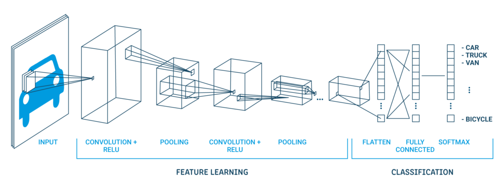
Convolutional neural network model using MNIST
In this section, we will create simple CNN models for MNIST that demonstrate convolutional layers, grouping layers and dropout layers.
Paso 1: import all necessary libraries
import numpy as np
from keras.models import Sequential
from keras.layers import Dense
from keras.utils import np_utils
from keras.layers import Dropout
from keras.layers import Flatten
from keras.layers.convolutional import Conv2D
from keras.layers.convolutional import MaxPooling2D
Paso 2: Set up the seed for reproducibility and load the MNIST data
seed=10
np.random.seed(seed)
(X_train,y_train), (X_test, y_test)= mnist.load_data()
Paso 3: convert data to float values
X_train=X_train.reshape(X_train.shape[0], 1,28,28).astype('float32')
X_test=X_test.reshape(X_test.shape[0], 1,28,28).astype('float32')
Paso 4: normalize data
X_train=X_train/255
X_test=X_test/255
y_train= np_utils.to_categorical(y_train)
y_test= np_utils.to_categorical(y_test)
num_classes=y_train.shape[1]
print(num_classes)
A classic CNN architecture looks like below:
| Output layer (10 Departures) |
| Hidden cloak (128 neurons) |
| Flat layer |
| Cloak of Abandonment 20% |
| Maximum grouping layer 2 × 2 |
| convolutional cover 32 maps, 5 × 5 |
| Visible layer 1x28x28 |
The first hidden layer is a convolutional layer called Convolution2D. Dispose of 32 feature maps with size 5 × 5 and grinding function. This is the input layer. The following is the pooling layer that takes the maximum value called MaxPooling2D. In this model, is configured as a pool size of 2 × 2.
En la capa de abandono ocurre la regularizationRegularization is an administrative process that seeks to formalize the situation of people or entities that operate outside the legal framework. This procedure is essential to guarantee rights and duties, as well as to promote social and economic inclusion. In many countries, Regularization is applied in migratory contexts, labor and tax, allowing those who are in irregular situations to access benefits and protect themselves from possible sanctions..... It is set to randomly exclude the 20% layer neurons to avoid overfitting. The fifth layer is the flattened layer that converts the 2D matrix data into a vector called Flatten. Allows the output to be fully processed by a fully connected standard layer.
Then, the fully connected layer is used with 128 neuronas y la wake functionThe activation function is a key component in neural networks, since it determines the output of a neuron based on its input. Its main purpose is to introduce nonlinearities into the model, allowing you to learn complex patterns in data. There are various activation functions, like the sigmoid, ReLU and tanh, each with particular characteristics that affect the performance of the model in different applications.... del rectificador. Finally, the output layer has 10 neurons for 10 classes and a softmax trigger function to generate probability-like predictions for each class.
Paso 5: run the model
def cnn_model():
    model=Sequential()
    model.add(Conv2D(32,5,5, padding='same',input_shape=(1,28,28), activation = 'reread'))
    model.add(MaxPooling2D(pool_size=(2,2), padding='same'))
    model.add(Dropout(0.2))
    model.add(Flatten())
    model.add(Dense(128, activation = 'reread'))
    model.add(Dense(num_classes, activation='softmax'))
    model.compile(loss="categorical_crossentropy", optimizer="adam", metrics=['accuracy'])
    return model
model=cnn_model()
model.fit(X_train, y_train, validation_data=(X_test,y_test),epochs=10, batch_size=200, verbose=2)
score= model.evaluate(X_test, y_test, verbose=0)
print('The error is: %.2f%%'%(100-score[1]*100))
Production:
Epoch 1/10
300/300 - 2s - loss: 0.7825 - accuracy: 0.7637 - val_loss: 0.3071 - val_accuracy: 0.9069
Epoch 2/10
300/300 - 1s - loss: 0.3505 - accuracy: 0.8908 - val_loss: 0.2192 - val_accuracy: 0.9336
Epoch 3/10
300/300 - 1s - loss: 0.2768 - accuracy: 0.9126 - val_loss: 0.1771 - val_accuracy: 0.9426
Epoch 4/10
300/300 - 1s - loss: 0.2392 - accuracy: 0.9251 - val_loss: 0.1508 - val_accuracy: 0.9537
Epoch 5/10
300/300 - 1s - loss: 0.2164 - accuracy: 0.9325 - val_loss: 0.1423 - val_accuracy: 0.9546
Epoch 6/10
300/300 - 1s - loss: 0.1997 - accuracy: 0.9380 - val_loss: 0.1279 - val_accuracy: 0.9607
Epoch 7/10
300/300 - 1s - loss: 0.1856 - accuracy: 0.9415 - val_loss: 0.1179 - val_accuracy: 0.9632
Epoch 8/10
300/300 - 1s - loss: 0.1777 - accuracy: 0.9433 - val_loss: 0.1119 - val_accuracy: 0.9642
Epoch 9/10
300/300 - 1s - loss: 0.1689 - accuracy: 0.9469 - val_loss: 0.1093 - val_accuracy: 0.9667
Epoch 10/10
300/300 - 1s - loss: 0.1605 - accuracy: 0.9493 - val_loss: 0.1053 - val_accuracy: 0.9659
The error is: 3.41%
In the model results, is visible as the number of epochs increases, improves accuracy. The mistake is 3.41%, lower error higher model precision.
Hope you enjoyed reading and feel free to use my code to test it for your purposes. What's more, if there is any comment on the code or just the blog post, feel free to contact me at [email protected]
Media shown in this CNN image processing article is not the property of DataPeaker and is used at the author's discretion.


