
This article was published as part of the Data Science Blogathon
Introduction
. Un problema de regresión es cuando la variableIn statistics and mathematics, a "variable" is a symbol that represents a value that can change or vary. There are different types of variables, and qualitative, that describe non-numerical characteristics, and quantitative, representing numerical quantities. Variables are fundamental in experiments and studies, since they allow the analysis of relationships and patterns between different elements, facilitating the understanding of complex phenomena.... de salida es un valor real o continuo.
- What is a regression?
- Regression types.
- What is the mean of the linear regression and the importance of the linear regression?
- Importancia de la función de costo y el descenso del gradientGradient is a term used in various fields, such as mathematics and computer science, to describe a continuous variation of values. In mathematics, refers to the rate of change of a function, while in graphic design, Applies to color transition. This concept is essential to understand phenomena such as optimization in algorithms and visual representation of data, allowing a better interpretation and analysis in... en una regresión lineal.
- Impact of different values on the learning rate.
- Implement Linear Regression Use Case With Python Code.
What is a regression?
In regression, we plot a graph between the variables that best fit the given data points. Machine learning model can provide predictions on data. En palabras liberal, “Regression displays a line or curve that passes through all the data points on a target prediction chart in such a way that the vertical distance between the data points and the regression line is minimal”. It is mainly used to predict, predict, model time series and determine the causal-effect relationship between variables.
Types of regression models
- Linear regression
- Polynomial regression
- Logistic regression
Linear regression
Linear regression is a simple and silent statistical regression method used for predictive analysis and shows the relationship between continuous variables. Linear regression shows the linear relationship between the independent variable (X axis) and the dependent variable (Axis y), consequently called linear regression. If there is a single input variable (x), said linear regression is called Simple linear regression. And if there is more than one input variable, said linear regression is called multiple linear regression. The linear regression model gives a sloping straight line that describes the relationship within the variables.
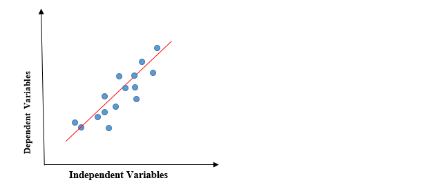
The previous graph presents the linear relationship between the dependent variable and the independent variables. When the value of x (independent variable) increases, the value of y (dependent variable) is also increasing. The red line is known as the straight line of best fit.. Based on the given data points, we try to draw a line that better models the points.
To Calculate Linear Regression of Line of Best Fit, a traditional slope-intercept form is used.

y = Dependent variable.
x = independent variable.
a0 = intersection of the line.
a1 = Coefficient of linear regression.
Need for a linear regression
As mentioned earlier, linear regression estimates the relationship between a dependent variable and an independent variable. Let's understand this with a simple example:
Let's say we want to estimate an employee's salary based on the year of experience. You have the recent data of the company, which indicates that the relationship between experience and salary. Here the year of experience is an independent variable and an employee's salary is a dependent variable., since an employee's salary depends on an employee's experience. With this information, we can predict the future salary of the employee based on current and past information.
A regression line can be a positive linear relationship or a negative linear relationship.
Positive linear relationship
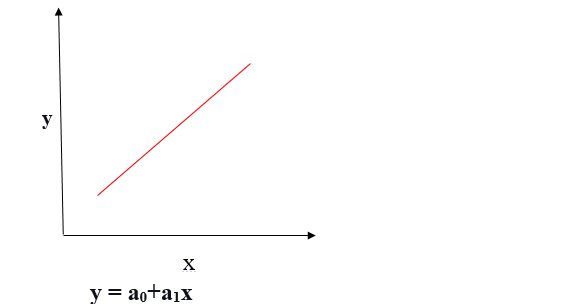
If the dependent variable expands on the Y axis and the independent variable progresses on the X axis, this relationship is called a positive linear relationship.
Negative linear relationship
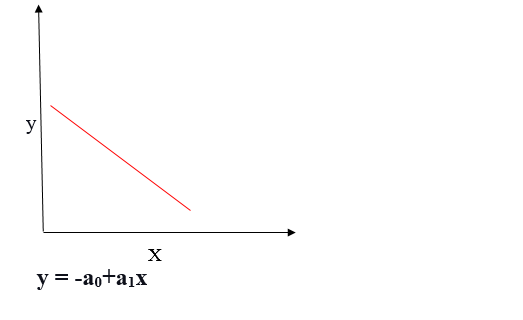
If the dependent variable decreases on the Y axis and the independent variable increases on the X axis, this relationship is called a negative linear relationship.
The objective of the linear regression algorithm is to obtain the best values for a0 and a1 to find the line of best fit. The line of best fit should have the least error, which means that the error between the predicted values and the actual values should be minimized.
Cost function
The cost function helps determine the best possible values for a0 and a1, which provides the line of best fit for the data points.
The cost function optimizes the regression coefficients or weights and measures how well a linear regression model is performing. The cost function is used to find the precision of the mapping function which maps the input variable to the output variable. This mapping function is also known as the hypothesis function.
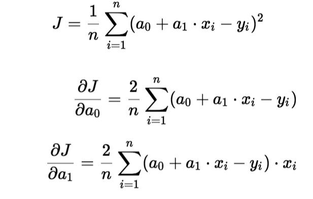
In linear regression, Root mean square error (MSE) The cost function is used, which is the average of the squared error that occurred between the predicted values and the actual values.
By simple linear equation y = mx + b we can calculate MSE as:
Let's y = real values, YI = predicted values

Using the MSE function, we will change the values of a0 and a1 so that the MSE value is set to the minimum. ParametersThe "parameters" are variables or criteria that are used to define, measure or evaluate a phenomenon or system. In various fields such as statistics, Computer Science and Scientific Research, Parameters are critical to establishing norms and standards that guide data analysis and interpretation. Their proper selection and handling are crucial to obtain accurate and relevant results in any study or project.... of the model xi, b (a0,a1) can be manipulated to minimize cost function. These parameters can be determined using the gradient descent method so that the value of the cost function is minimal.
Gradient descent
Gradient descent is a method of updating a0 and a1 to minimize the cost function (MSE). A regression model uses gradient descent to update the coefficients of the line (a0, a1 => xi, b) by reducing the cost function using a random selection of coefficient values and then iteratively updating the values to reach the minimum cost function.
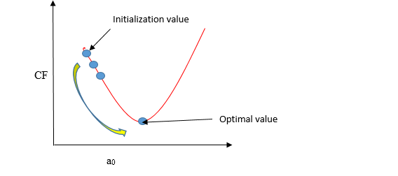
Imagine a U-shaped well. You are standing at the highest point of the well and your goal is to reach the bottom of the well. There is a treasure, and you can only take a discrete number of steps to get to the bottom. If you decide to take one step at a time, you'll eventually reach the bottom of the well, but this will take longer. If you choose to take longer steps each time, can arrive earlier, but there is a possibility that it may go over the bottom of the well and not near the bottom. In the gradient descent algorithm, the number of steps you take is the learning rate, and this decides how fast the algorithm converges to the minima.
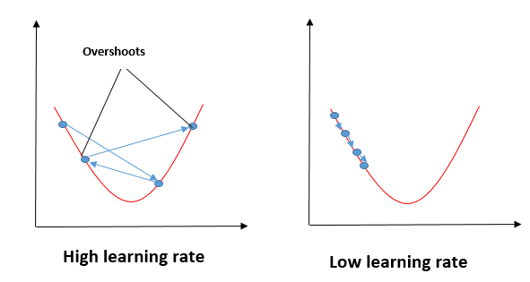
To update a0 and a1, we take gradients from the cost function. To find these gradients, we take partial derivatives for a0 and a1.
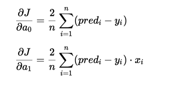
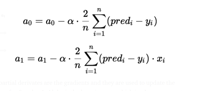
The partial derivatives are the gradients and are used to update the values of a0 and a1. Alpha is the learning rate.
Impact of different values for the learning rate
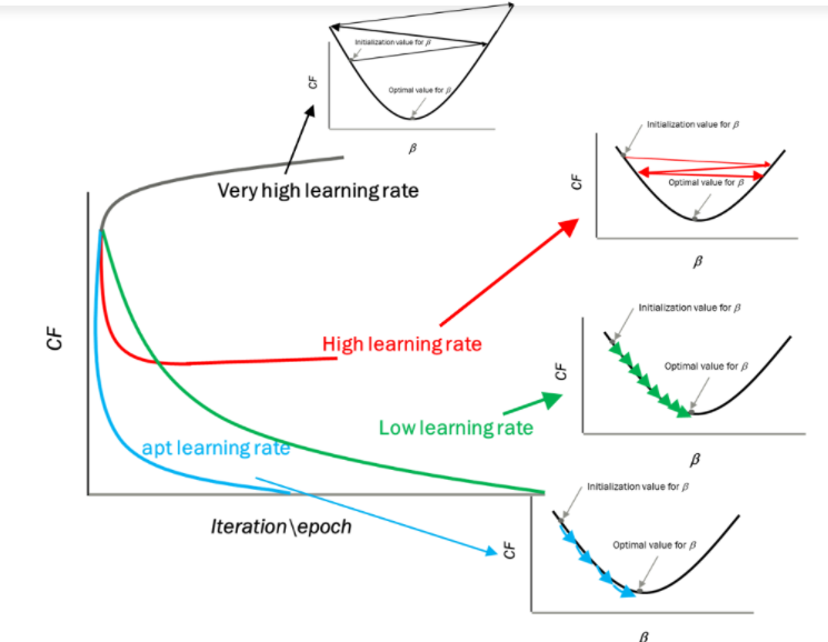
Source: mygreatleaning.com
The blue line represents the optimal value of the learning rate and the value of the cost function is minimized in a few iterations. The green line represents if the learning rate is less than the optimal value, then the number of iterations required is high to minimize the cost function. If the selected learning rate is very high, the cost function could continue to increase with iterations and saturate to a value higher than the minimum value, the one represented by a red and black line.
Case of use
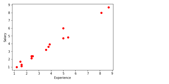
In this, I'll take random numbers for the dependent variable (salary) and an independent variable (experience) and I will predict the impact of one year of experience on salary.
Steps to implement the linear regression model
import some required libraries
import matplotlib.pyplot as plt
import pandas as pd
import numpy as np
Define the dataset
x= np.array([2.4,5.0,1.5,3.8,8.7,3.6,1.2,8.1,2.5,5,1.6,1.6,2.4,3.9,5.4])
y = np.array([2.1,4.7,1.7,3.6,8.7,3.2,1.0,8.0,2.4,6,1.1,1.3,2.4,3.9,4.8])
n = np.size(x)
Plot the data points
plt.scatter(experience,salary, color="red")
plt.xlabel("Experience")
plt.ylabel("Salary")
plt.show()
The main function for calculating coefficient values.
- Initialize the parameters.
- Predict the value of a dependent variable given an independent variable.
- Calculate the error in the prediction for all data points.
- Calculate the partial derivative wrt a0 and a1.
- Calculate the cost of each number and add them up.
- Update the values of a0 and a1.
#initialize the parameters
a0 = 0                  #intercept
a1 = 0                  #Slop
lr = 0.0001             #Learning rate
iterations = 1000       # Number of iterations
error = []              # Error array to calculate cost for each iterations.
for itr in range(iterations):
    error_cost = 0
    cost_a0 = 0
    cost_a1 = 0
    for i in range(len(experience)):
        y_pred = a0+a1*experience[i]   # predict value for given x
        error_cost = error_cost +(salary[i]-y_pred)**2
        for j in range(len(experience)):
            partial_wrt_a0 = -2 *(salary[j] - (a0 + a1*experience[j]))                #partial derivative w.r.t a0
            partial_wrt_a1 = (-2*experience[j])*(salary[j]-(a0 + a1*experience[j]))   #partial derivative w.r.t a1
            cost_a0 = cost_a0 + partial_wrt_a0      #calculate cost for each number and add
            cost_a1 = cost_a1 + partial_wrt_a1      #calculate cost for each number and add
        a0 = a0 - lr * cost_a0    #update a0
        a1 = a1 - lr * cost_a1    #update a1
        print(itr,a0, a1)          #Check iteration and updated a0 and a1
    error.append(error_cost)      #Append the data in array
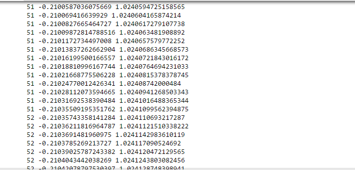
In a rough iteration of 50-60, we obtained the value of a0 and a1.
print(a0)
print(a1)

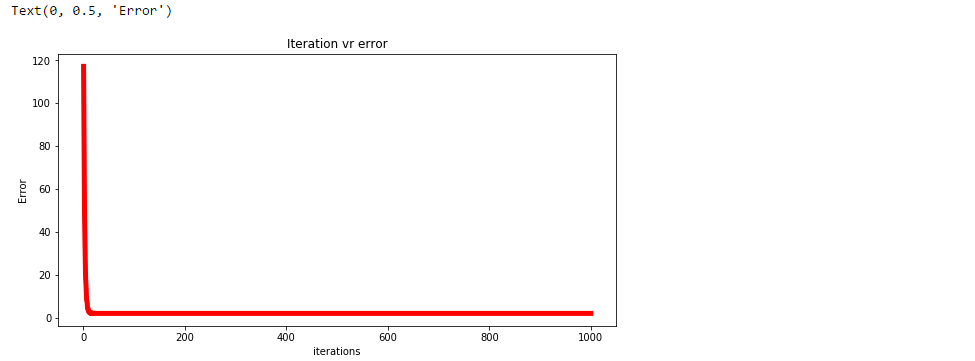
Plot the error for each iteration.
plt.figure(figsize=(10,5))
plt.plot(np.arange(1,len(error)+1),error,color="red",linewidth = 5)
plt.title("Iteration vr error")
plt.xlabel("iterations")
plt.ylabel("Error")
Predict values.
pred = a0+a1*experience
print(pred)

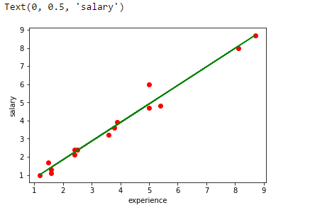
Draw the regression line.
plt.scatter(experience,salary,color="red")
plt.plot(experience,pred, color="green")
plt.xlabel("experience")
plt.ylabel("salary")
Analyze the performance of the model by calculating the root mean square error.
error1 = salary - pred
se = np.sum(error1 ** 2)
mse = se/n
print("mean squared error is", mse)

Use the scikit library to confirm the above steps.
from sklearn.linear_model import LinearRegression
from sklearn.metrics import mean_squared_error
experience = experience.reshape(-1,1)
model = LinearRegression()
model.fit(experience,salary)
salary_pred = model.predict(experience)
Mse = mean_squared_error(salary, salary_pred)
print('slop', model.coef_)
print("Intercept", model.intercept_)
print("MSE", Mse)

Summary
In regression, we plot a graph between the variables that best fit the given data points. Linear regression shows the linear relationship between the independent variable (X axis) and the dependent variable (Axis y).To Calculate Linear Regression of Line of Best Fit, a traditional slope-intercept form is used. A regression line can be a positive linear relationship or a negative linear relationship.
The goal of the linear regression algorithm is to obtain the best values for a0 and a1 to find the line of best fit and the line of best fit must have the smallest error. In linear regression, Root mean square error (MSE) the cost function is used, that helps determine the best possible values for a0 and a1, which provides the line of best fit for the data points. Using the MSE function, we will change the values of a0 and a1 so that the MSE value is set to the minimum. Gradient descent is a method of updating a0 and a1 to minimize the cost function (MSE)
The media shown in this article is not the property of DataPeaker and is used at the author's discretion.





