
This article was published as part of the Data Science Blogathon.
Warning: this article is for absolute beginners, I guess you just entered the field of machine learning with some high school math skills and some basic coding, but that's not even mandatory.
Introduction
Linear regression is the most basic supervised machine learning algorithm. Monitor in the sense that the algorithm can answer your question based on tagged data that you feed to the algorithm. The answer would be how to predict house prices, classify dogs versus cats. Here we are going to talk about a regression task using Linear Regression. In the end, we are going to predict house prices based on the area of the house.
I don't want to bore you by throwing out all the words of machine learning jargon, at first, so let me start with the most basic linear equation. (y = mx + b) that we all know from our school days.
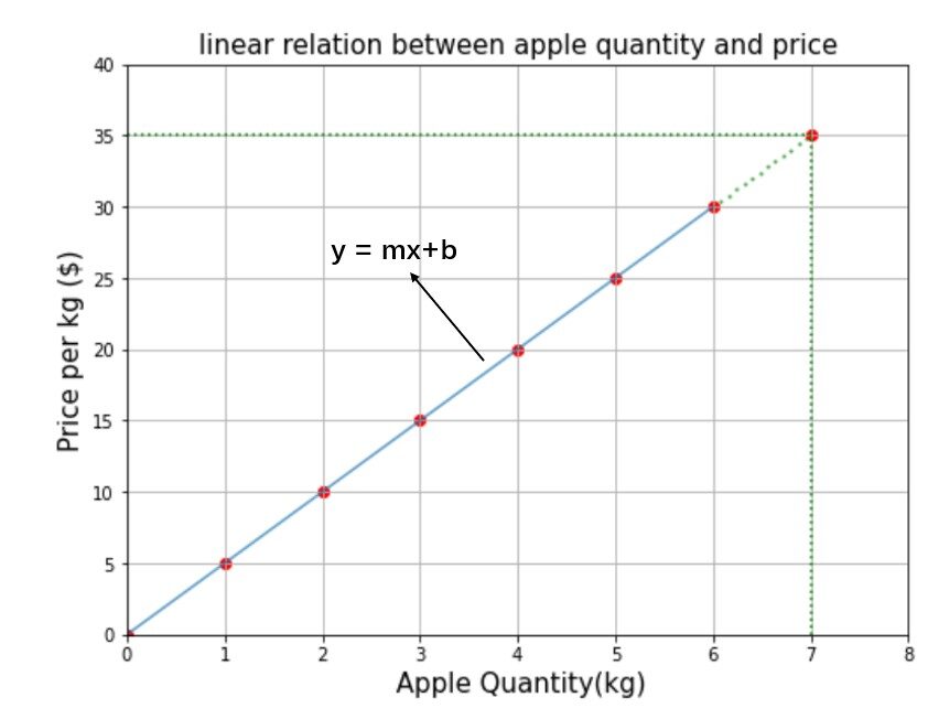
The figure"Figure" is a term that is used in various contexts, From art to anatomy. In the artistic field, refers to the representation of human or animal forms in sculptures and paintings. In anatomy, designates the shape and structure of the body. What's more, in mathematics, "figure" it is related to geometric shapes. Its versatility makes it a fundamental concept in multiple disciplines.... anterior muestra la relación entre la cantidad de manzana y el precio de costo. How much do you have to pay for 7 kg of apples? I know its easy. And 1 kg costs 5 $, then 7 kg cost 7 * 5 = 35 $ or it will just draw a perpendicular line from the point 7 along the y-axis until it touches the linear equation and the corresponding value on the y-axis is the answer as shown. by the green dotted line on the graph. But we are going to solve using the formula of a linear equation.

Now, if I have to find the price of 9,5 kg of apple, according to our model mx + b = 5 * 9.5 + 0 = $ 47.5 is the answer. At this stage, you may have understood that metro Y B are the main ingredients of the linear equation or in other words metro Y B They are called parametersThe "parameters" are variables or criteria that are used to define, measure or evaluate a phenomenon or system. In various fields such as statistics, Computer Science and Scientific Research, Parameters are critical to establishing norms and standards that guide data analysis and interpretation. Their proper selection and handling are crucial to obtain accurate and relevant results in any study or project.....
Unfortunately, this is not the machine learning problem nor is the linear equation a prediction algorithm, but fortunately the linear regression generates the result in the same way that the linear equation does. The main purpose of the linear regression algorithm is to find the value of metro Y B that fit the model and after that metro Y b are used to predict the outcome of the given input data.
Predicting house prices
Now we are going to dig a little deeper into the solution of the regression problem. Look at the data samples or also named as ejemplos de trainingTraining is a systematic process designed to improve skills, physical knowledge or abilities. It is applied in various areas, like sport, Education and professional development. An effective training program includes goal planning, regular practice and evaluation of progress. Adaptation to individual needs and motivation are key factors in achieving successful and sustainable results in any discipline.... given in the figure below.
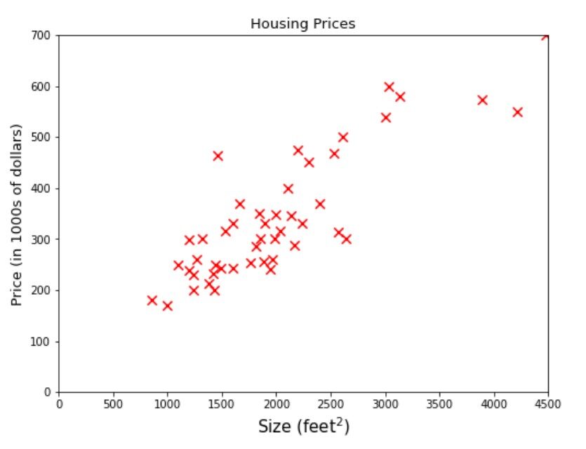
The name of a company A B C provides you with a data about him house size Y its price. The company requires providing them with a machine learning model that can predict house prices for any given Size. Let's say what would be the best estimated price for an area of 3000 square feet. If you are thinking of wrap a line somewhere between the dataset and draw a vertical line from 3000 on the x-axis until it touches the line and then the corresponding value on the y-axis, namely 470 would be the answer, then you are on the right track, is represented by the green dotted line in the figure below.
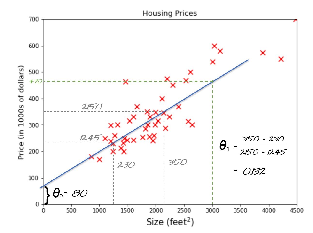
Let's do it another way, if we could find the equation of the line y = mx + b that we use to fit the data represented by the blue slanted line, then we can easily find the model that can predict house prices for any given area. . Based on machine learning jargon y = mx + b It's also called hypothesis function where myb can be represented by theta0 and theta1 respectively. theta0 is also called bias term and theta1, theta2, .. called pesos.
See the blue line in the picture above. When taking two samples that are touching or very close to the line, we can find the theta1 (pending) = 0.132 Y zero theta = 80 as the picture shows. Now we can use our hypothesis function to predict the house price for a size of 3000 square feet, namely. 80 + 3000 * 0,132 = 476. $ 476,000 could be the best estimated price for a house of 3000 square footage and this might be a reasonable way to prepare a machine learning model when you have just finished 50 samples and with only a feature (size).
But the real world data set could be on the order of thousands or even millions and the number of features could vary between (5–100) or even in thousands. At that time our intuition will not be useful to find thousands of parameters just by looking at a data set, that's why we need a machine learning algorithm to perform such a complex calculation. Have a cup of coffee, refresh yourself and come back again because from now on you will understand how the algorithm works and you will be introduced to a lot of new terminologies. Get prepared!!
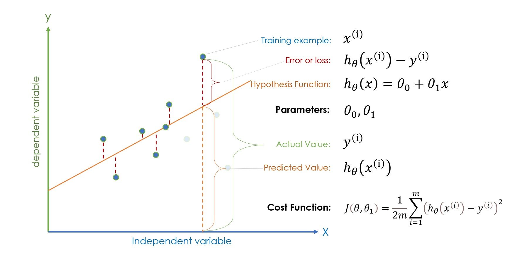
Note: (i) in the equation represents the i-th training example, not the power.
If the terminologies given in the figure above seem extraterrestrial to you, take a few minutes to familiarize yourself and try to find a connection to each term. If you know to a certain extent, let's move on. Once the parameter values, namely bias term Y theta1 randomly initialize, the hypothesis function is ready for prediction, and then the error (|predicted value – current value|) is calculated to check whether the randomly initialized parameter is giving the correct prediction or not.
If the error is too high, then the algorithm updates the parameters with a new value, if the error is high again, will update the parameters with the new value again. The algorithm continues this process until the error is minimized. To minimize error we have a special function called Decline of gradientGradient is a term used in various fields, such as mathematics and computer science, to describe a continuous variation of values. In mathematics, refers to the rate of change of a function, while in graphic design, Applies to color transition. This concept is essential to understand phenomena such as optimization in algorithms and visual representation of data, allowing a better interpretation and analysis in... but before that, let's understand what Cost function it is and how it works?
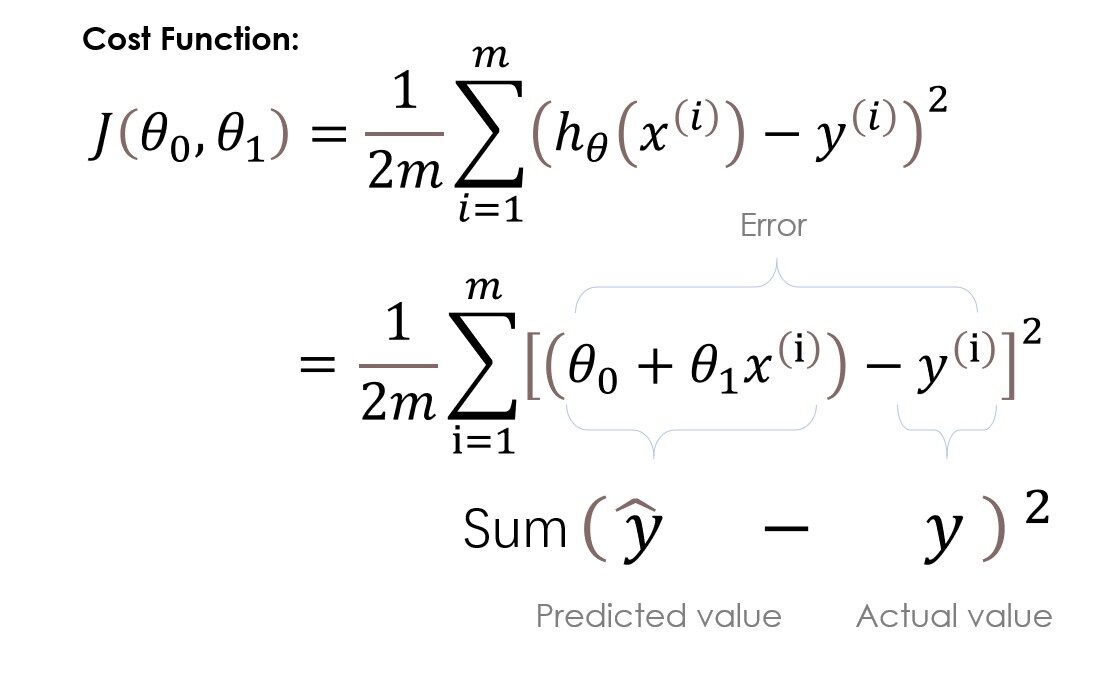
Here, in the cost function, we are trying to find the square of the differences between the predicted value and the actual value of each training example and then add all the differences together or in other words, we are finding the square of error of each training example and then summarize all errors together. The output we get is simply the mean squared error of a particular set of parameters. Ok, no more words, let's do the calculation. To simplify the calculation, we will use only one parameter theta1 and a very simple data set.
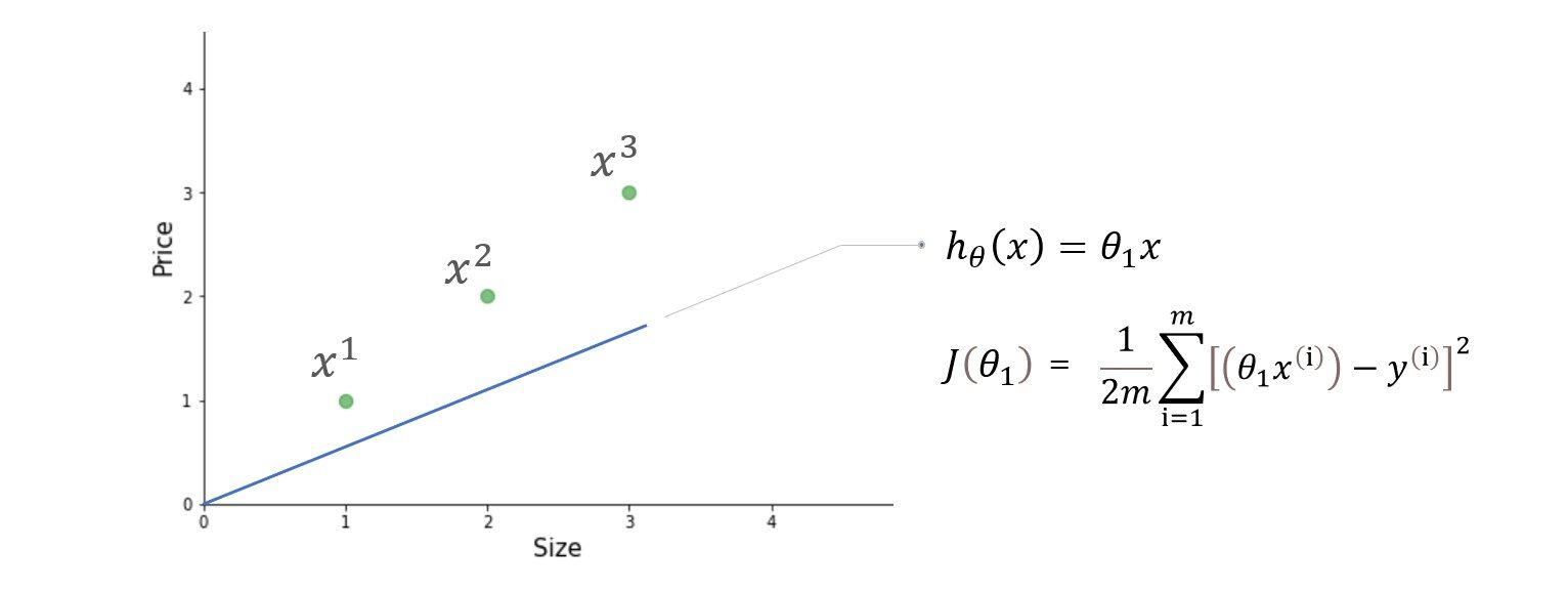

We have three training examples (X1 = 1, y1 = 1), (X2 = 2, y2 = 2) Y (X3 = 3, y3 = 3). the figure on the left is the hypothesis function and the figure on the right is the cost function graphed for different values of the parameter.
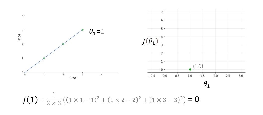
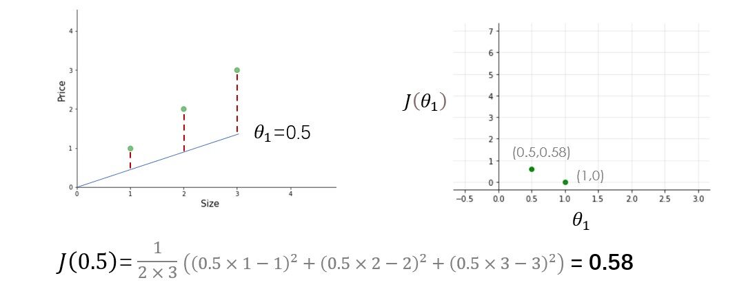
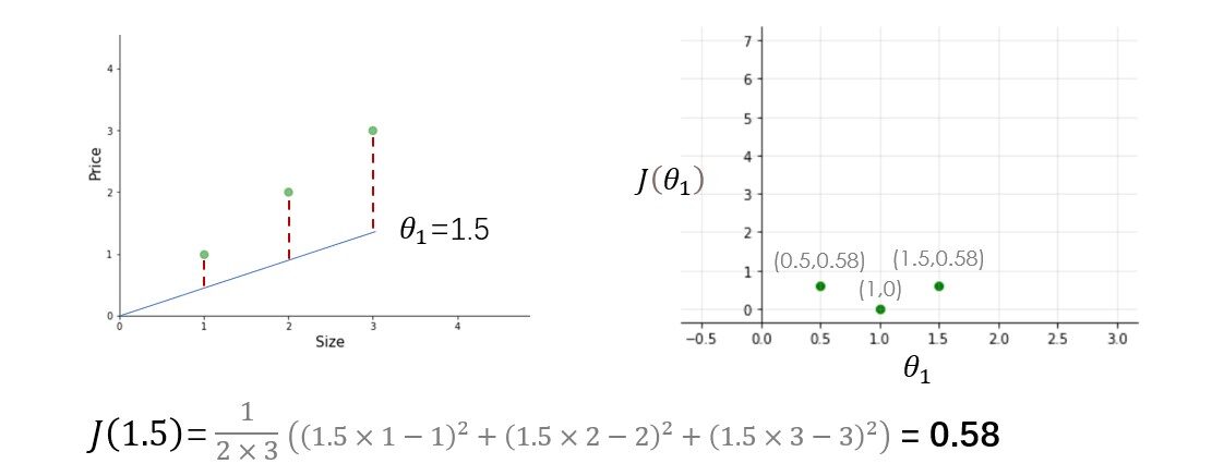
Try other values of theta1 yourself and calculate the cost of each value of theta1. Once I draw all these points, the cost function will look like a bowl-shaped curve as shown in the figure below.
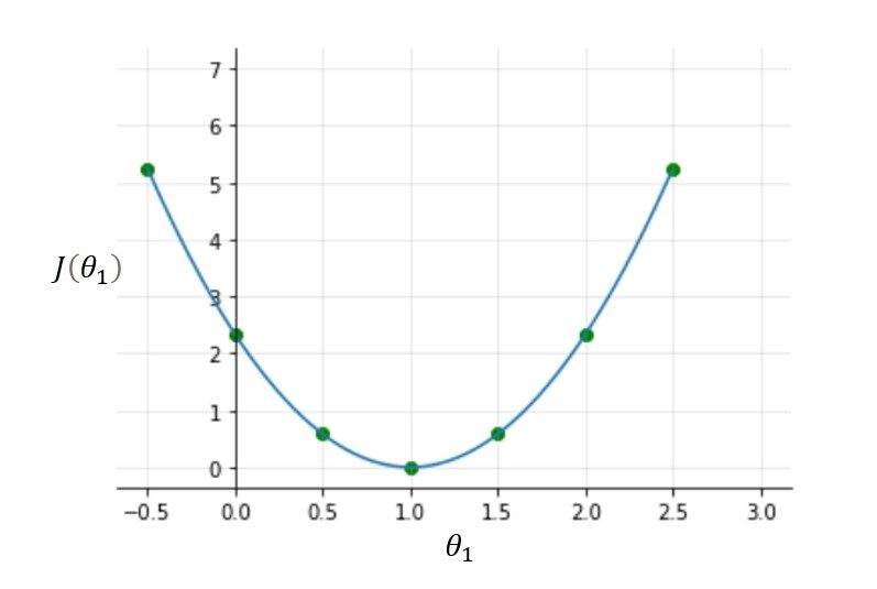
From the figure and the calculation, it is clear that the cost function is minimal at theta1 = 1 or at the bottom of the bowl-shaped curve. The purpose of all this hard work is not to calculate the minimum value of the cost function, we have a better way to do this, instead, we try to understand the relationship Between parameters, hypothesis function, Y cost function. Make sure you understand all of these concepts before proceeding any further..
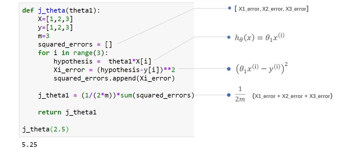
Coding cost function:
Gradient descent:
Why do we need a gradient descent?
- Soon to minimize the cost function, But how? We'll see
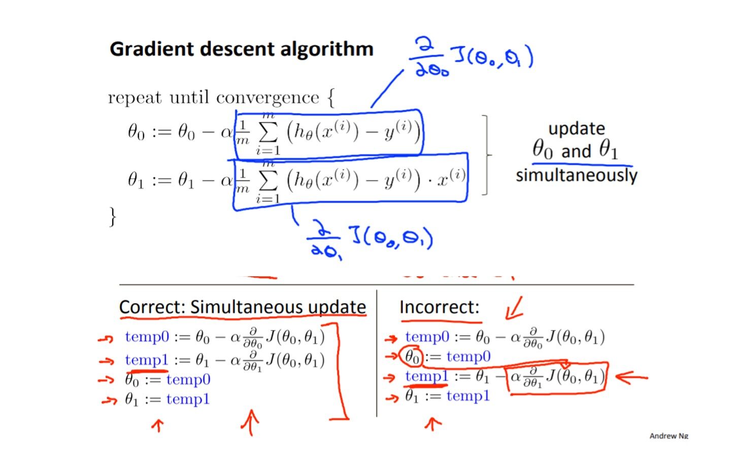
The cost function only works when you know the parameter values. In the sample example above, we manually choose the value of the parameters each time, but during algorithmic calculation, once the parameter values are randomly initialized, it is the descent of the gradient who has to decide which parameters. value to choose in the next iteration to minimize the error, it is the descent of the gradient who decides how much to increase or decrease the values of the parameters.
Analogy: How does Gradient Descent work?
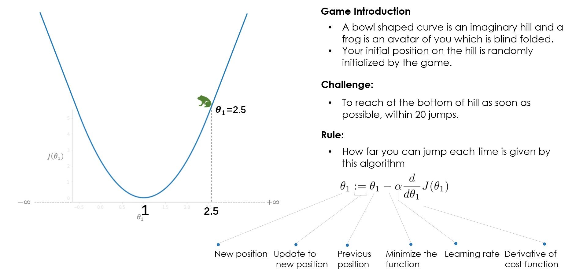
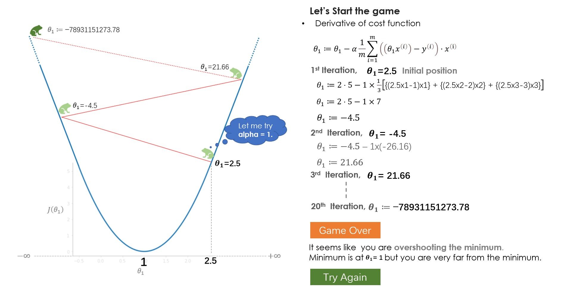
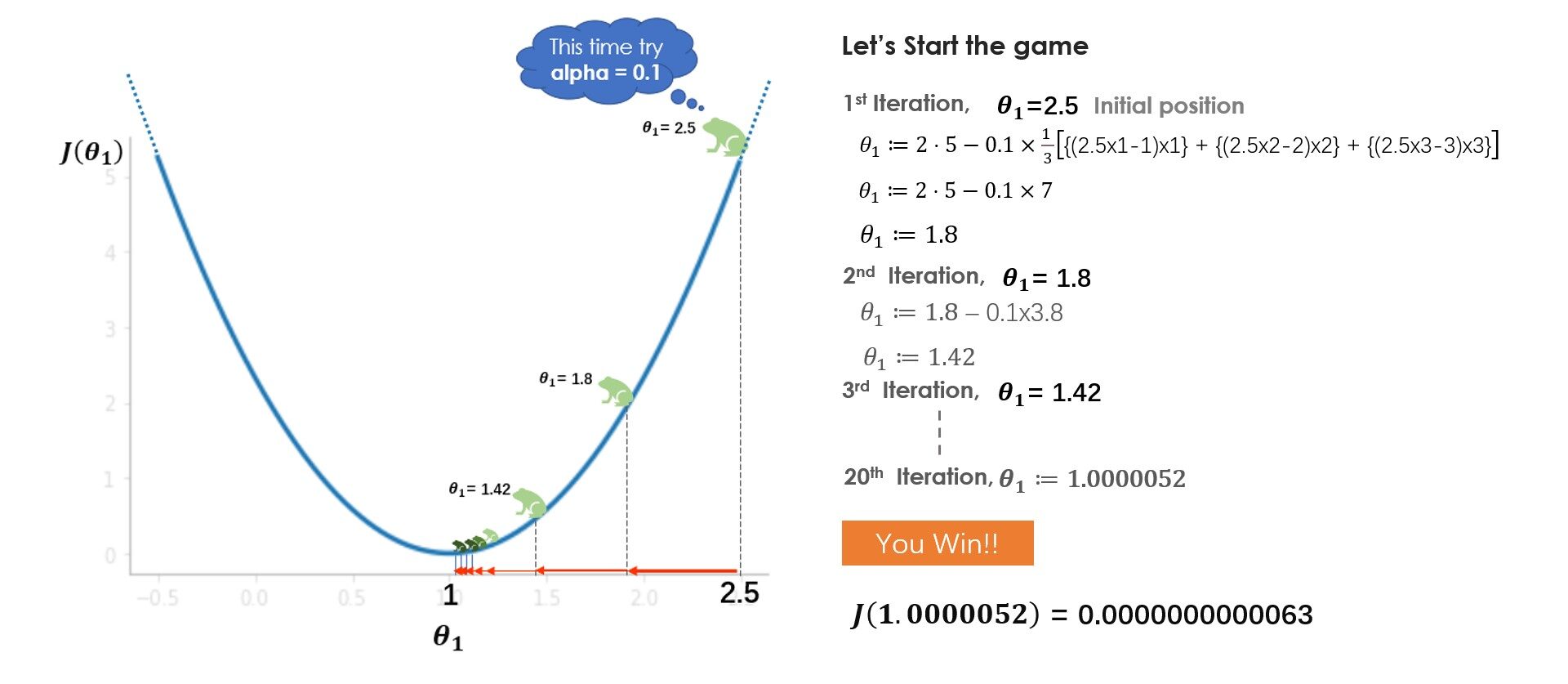
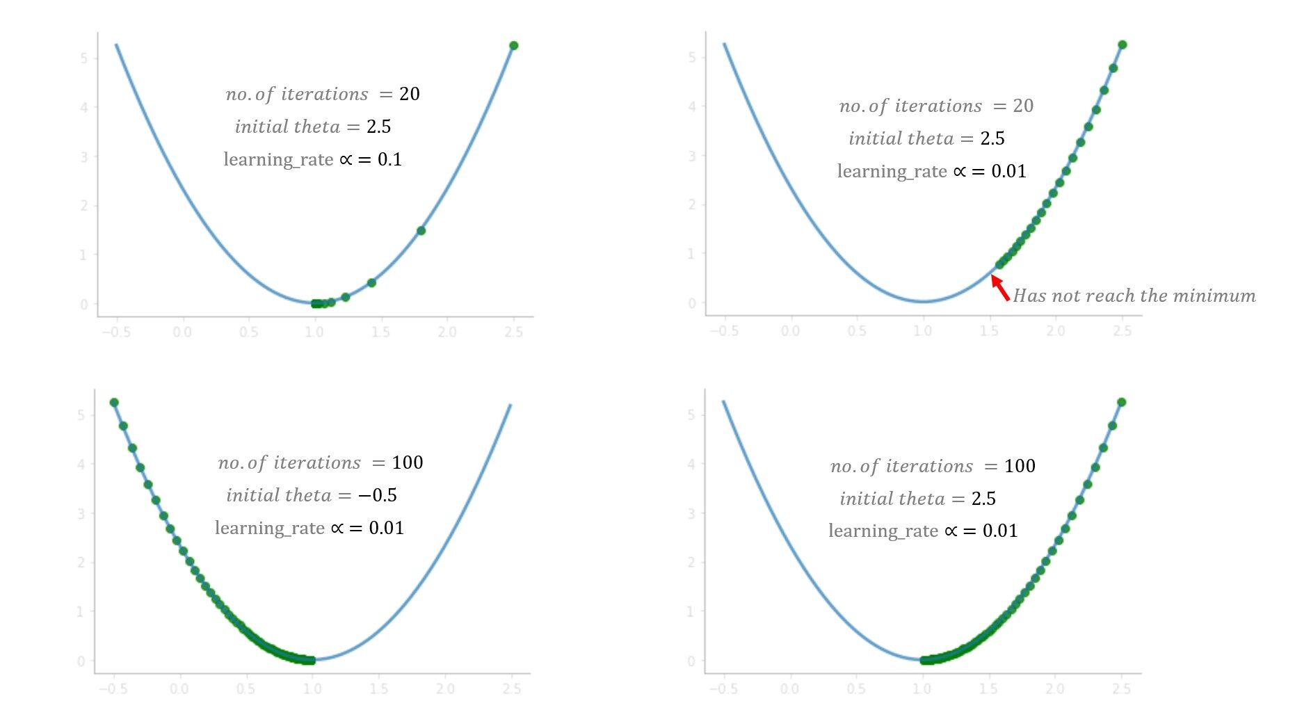
What did you learn from the game? In the beginning, you try a learning rate (alfa) = 1 but you don't reach the minimum, because the largest steps exceed the minimum. In the next game, you try with alpha = 0.1, and this time you managed to get to the bottom very safely. What if you had tried alpha = 0.01? Good, then, you will gradually go down but you will not reach the bottom, 20 jumps are not enough to get to the bottom with alpha = 0.01, 100 jumps might be enough. While solving a real world problem, normally an alpha between 0.01–0.1 should work fine, but it varies with the number of iterations the algorithm takes, some problems may require 100 or even 1000 iterations.
Based on these factors, you can try different alpha values. Although adjusting the alpha value is one of the important tasks to understand the algorithm, I suggest you look at other parts of the algorithm as well as the derived parts, the minus sign, update parameters and understand what the roles of your individuals are.
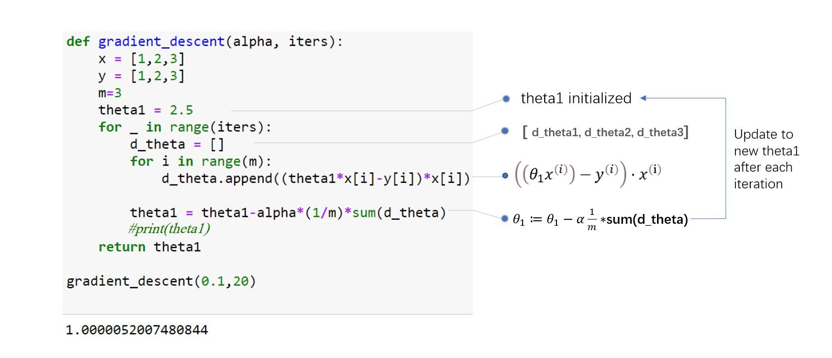
Coding gradient descent
Up to now, we are only using a single parameter to calculate the cost function and the algorithms. What does the cost function look like and how does the algorithm work when we have two or more parameters? See the figure below for an intuitive understanding. Imagine yourself somewhere on the top of the mountain and struggling to get down the base of the mountain blindfolded..
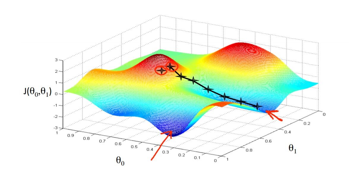
The principle of operation of the algorithm is the same for any number of parameters, it's just that the more the parameters the more the direction of the slope. In the above example of the bowl-shaped curve, we just need to observe the slope of theta1, but now the algorithm must look in both directions to minimize the cost function. Let's code and understand the algorithm. Please refer to the figure below for reference:
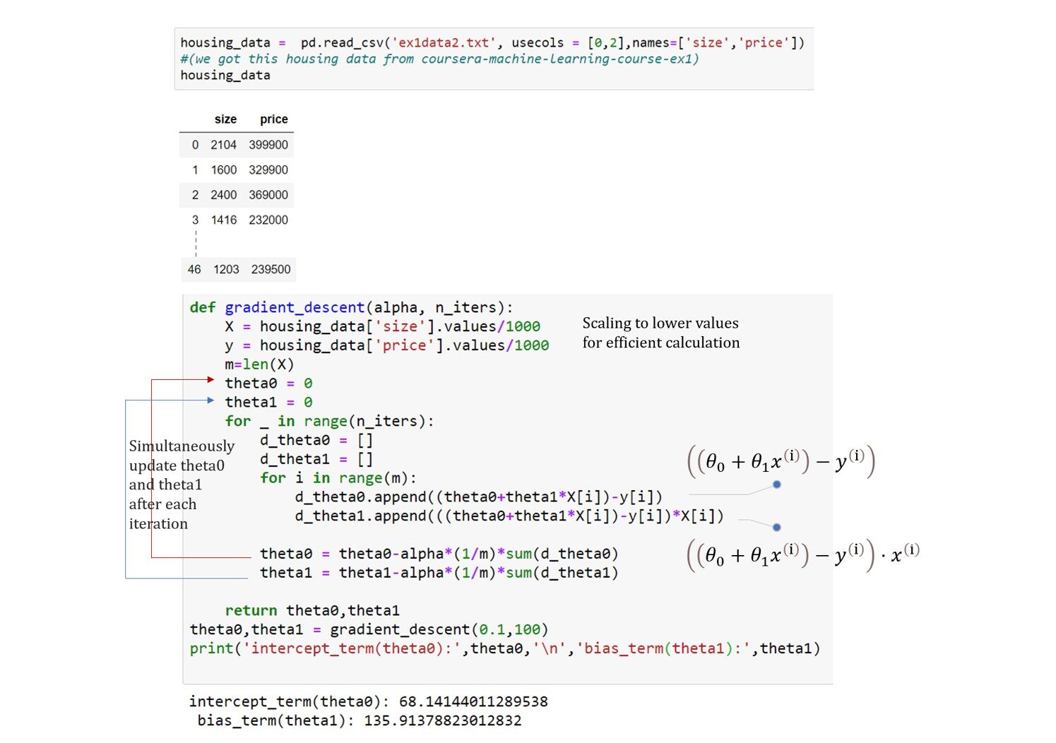
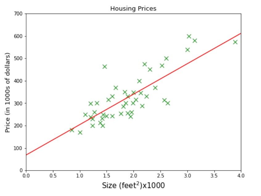

Here we go, our model predicts 475,88 * 1000 = $ 475,880 for house size 3 * 1000 square feet. It is very close to our prediction that we made at the beginning using our intuition.
Conclution
As a beginner, it can be a bit difficult to understand all the concepts of linear regression in such a short reading time. I wouldn't say you know everything about linear regression from this article. The purpose of this article is to make the algorithms understandable as simply as possible. Follow the resource link below for a better understanding. I hope you enjoyed reading the article. Thank you for reading.
Means:
code link
https://github.com/ravi235/LinearRegression
Gradient descent math
https://www.youtube.com/watch?v=jc2IthslyzM&ab_channel=TheCodingTrain
Linear Regression Andrew Ng
https://www.youtube.com/watch?v=kHwlB_j7Hkc&t=8s&ab_channel=ArtificialIntelligence-AllinOne





