This article was published as part of the Data Science Blogathon
In this article, We'll answer these basic questions and build a red neuronalNeural networks are computational models inspired by the functioning of the human brain. They use structures known as artificial neurons to process and learn from data. These networks are fundamental in the field of artificial intelligence, enabling significant advancements in tasks such as image recognition, Natural Language Processing and Time Series Prediction, among others. Their ability to learn complex patterns makes them powerful tools.. basic to perform linear regression.
What is a neural network?
The basic unit of the brain is known as a neuron, there are approximately 86 billion neurons in our nervous system that are connected to 10 ^ 14-10 ^ 15 synapse. meEach neuron receives a signal from the synapses and outputs it after processing the signal.. This idea is extracted from the brain to build a neural network.
Each neuron performs a scalar product between the inputs and the weights, add biases, applies a wake functionThe activation function is a key component in neural networks, since it determines the output of a neuron based on its input. Its main purpose is to introduce nonlinearities into the model, allowing you to learn complex patterns in data. There are various activation functions, like the sigmoid, ReLU and tanh, each with particular characteristics that affect the performance of the model in different applications.... and issues the outputs. When a large number of neurons are present together to give a large number of outputs, a neural layer is formed. Finally, multiple layers combine to form a neural network.
Arquitectura de red neuronal
Neural networks are formed when multiple neural layers combine with each other to give a network, or we can say that there are some layers whose outputs are inputs for other layers.
The most common type of layer to build a basic neural network is the fully connected layer, in which adjacent layers are completely paired and single-layer neurons are not connected to each other.
In the figure"Figure" is a term that is used in various contexts, From art to anatomy. In the artistic field, refers to the representation of human or animal forms in sculptures and paintings. In anatomy, designates the shape and structure of the body. What's more, in mathematics, "figure" it is related to geometric shapes. Its versatility makes it a fundamental concept in multiple disciplines.... anterior, neural networks are used to classify data points into three categories.
Naming conventions. When the N-layer neural network, We don't count the input layerThe "input layer" refers to the initial level in a data analysis process or in neural network architectures. Its main function is to receive and process raw information before it is transformed by subsequent layers. In the context of machine learning, Proper configuration of the input layer is crucial to ensure the effectiveness of the model and optimize its performance in specific tasks..... Therefore, a single-layer neural network describes a network with no hidden layers (input is mapped directly to output). In the case of our code, we are going to use a single layer neural network, namely, we don't have a hidden layer.
Output layerThe "Output layer" is a concept used in the field of information technology and systems design. It refers to the last layer of a software model or architecture that is responsible for presenting the results to the end user. This layer is crucial for the user experience, since it allows direct interaction with the system and the visualization of processed data..... Unlike all layers in a neural network, neurons in the output layer commonly do not have a firing function (or you can think they have a linear identity activation function). This is because the last layer of output is usually taken to represent the class scores (for instance, in the classification), which are arbitrary real value numbers or some kind of real value target (for instance, in regression). Since we are doing the regression using a single layer, we don't have any activation function.
Neural network sizing. The two metrics that people commonly use to measure the size of neural networks are the number of neurons or, more commonly, The number of parametersThe "parameters" are variables or criteria that are used to define, measure or evaluate a phenomenon or system. In various fields such as statistics, Computer Science and Scientific Research, Parameters are critical to establishing norms and standards that guide data analysis and interpretation. Their proper selection and handling are crucial to obtain accurate and relevant results in any study or project.....
Libraries
We will use three basic libraries for this model, numpy, matplotlib and TensorFlow.
- Numpy: this adds support for large, multidimensional arrays and arrays, along with a large collection of high-level math functions. In our case, we are going to generate data with the help of Numpy.
- Matplotlib: this is a plotting library for python, we will visualize the final results using graphs in Matplotlib.
- Tensorflow: This library has a particular focus on the trainingTraining is a systematic process designed to improve skills, physical knowledge or abilities. It is applied in various areas, like sport, Education and professional development. An effective training program includes goal planning, regular practice and evaluation of progress. Adaptation to individual needs and motivation are key factors in achieving successful and sustainable results in any discipline.... and deep neural network inference. We can directly import the layers and train, test functions without having to write the whole program.
import numpy as np
import matplotlib.pyplot as plt
import tensorflow as tf
Generating data
We can generate our own numerical data for this process using the np.unifrom function () that generates uniform data. Here, we are using two input variables xs and zs, adding some noise to randomize the data points and, Finally, the variableIn statistics and mathematics, a "variable" is a symbol that represents a value that can change or vary. There are different types of variables, and qualitative, that describe non-numerical characteristics, and quantitative, representing numerical quantities. Variables are fundamental in experiments and studies, since they allow the analysis of relationships and patterns between different elements, facilitating the understanding of complex phenomena.... Target is defined as y = 2 * xs-3 * zs + 5 + noise. The size of the data set is 1000.
observations=1000
xs=np.random.uniform(-10,10,(observations,1))
zs=np.random.uniform(-10,10,(observations,1))
generated_inputs=np.column_stack((xs,zs))
noise=np.random.uniform(-10,10,(observations,1))
generated_target=2*xs-3*zs+5+noise
After generating the data, save them to an .npz file, so they can be used for training.
np. know('TF_intro',input=generated_inputs,targets=generated_target)
training_data=np.load('TF_intro.npz')
Our goal is to get the final weights as close as possible to the actual weights, namely [2,-3].
Defining the model
Here, we will use the dense layerThe dense layer is a geological formation that is characterized by its high compactness and resistance. It is commonly found underground, where it acts as a barrier to the flow of water and other fluids. Its composition varies, but it usually includes heavy minerals, which gives it unique properties. This layer is crucial in geological engineering and water resources studies, since it influences the availability and quality of water.. to make the model and import the drop of the gradientGradient is a term used in various fields, such as mathematics and computer science, to describe a continuous variation of values. In mathematics, refers to the rate of change of a function, while in graphic design, Applies to color transition. This concept is essential to understand phenomena such as optimization in algorithms and visual representation of data, allowing a better interpretation and analysis in... Keras Optimizer Stochastic.
A gradient is the slope of a function. Measures the degree to which one variable changes with changes in another variable. Mathematically, gradient descent is a convex function whose output is the partial derivation of a set of parameters from its inputs. The higher the slope, the steeper the slope.
Starting from an initial value, Gradient Descent runs iteratively to find the optimal values of the parameters to find the minimum possible value for the given cost function. The word “stochastic” refers to a random probability system or process. Therefore, en Stochastic Gradient Descent, some samples are randomly selected, instead of the dataset for each iteration.
Given the, the entrance has 2 variables, inlet size = 2 and output size = 1.
We set the learning rate at 0.02, which is neither too high nor too low, and the epoch value = 100.
input_size=2
output_size=1
models = tf.keras.Sequential([
                             tf.hard.layers.Dense(output_size)
                            ])
custom_optimizer=tf.keras.optimizers.SGD(learning_rate=0.02)
models.compile(optimizer=custom_optimizer,loss="mean_squared_error")
models.fit(training_data['input'],training_data['targets'],epochs=100,verbose=1)
Get weights and biases
We can print the predicted values of weights and biases and also store them.
models.layers[0].get_weights()
[array([[ 1.3665189],
        [-3.1609795]], dtype=float32), array([4.9344487], dtype=float32)]
Here, the first matrix represents the weights and the second matrix represents the biases. We can clearly see that the predicted values of the weights are very close to the actual value of the weights..
weights=models.layers[0].get_weights()[0]
bias=models.layers[0].get_weights()[1]
Prediction and precision
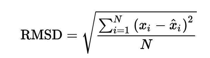
After prediction using the given weights and biases, a final RMSE score of 0.02866, which is quite low.
RMSE is defined as the root mean square error. The root mean square error takes the difference for each observed and predicted value. The formula for the RMSE error is given as:
https://www.google.com/search?q=rmse+formula&oq=RMSE+form&aqs=chrome.0.0i433j0j69i57j0l7.4779j0j7&sourceid=chrome&ie=UTF-8
 |
|
|
|
 |
|
|
|
 |
|
|
|
 |
|
|
out=training_data['targets'].round(1)
from sklearn.metrics import mean_squared_error
mean_squared_error(generated_target, out, squared=False)
If we plot the predicted data in a Dispersion diagramThe scatter plot is a graphical tool used in statistics to visualize the relationship between two variables. It consists of a set of points in a Cartesian plane, where each point represents a pair of values corresponding to the variables analyzed. This type of chart allows you to identify patterns, Trends and possible correlations, facilitating data interpretation and decision-making based on the visual information presented...., we get a graph like this:
plt.scatter(np.squeeze(models.predict_on_batch(training_data['input'])),np.squeeze(training_data['targets']),c="#88c999")
plt.xlabel('Input')
plt.ylabel('Predicted Output')
plt.show()
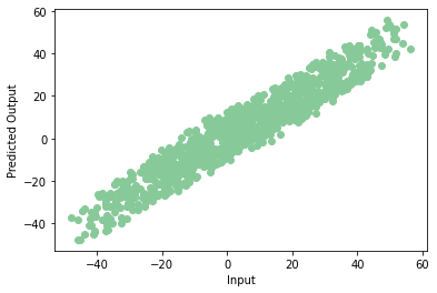
Hurray! Our model is trained correctly with very few errors. This is the end of your first neural network. Note that each time we train the model we can obtain a different precision value, but they won't differ much.
Thank you for reading! You can contact me at [email protected]
The media shown in this article is not the property of DataPeaker and is used at the author's discretion.


