
This article was published as part of the Data Science Blogathon.
Introduction
Interested in predictive analytics? Later, research artificial intelligence, machine learning and deep learningDeep learning, A subdiscipline of artificial intelligence, relies on artificial neural networks to analyze and process large volumes of data. This technique allows machines to learn patterns and perform complex tasks, such as speech recognition and computer vision. Its ability to continuously improve as more data is provided to it makes it a key tool in various industries, from health.... .
If you are on the path of learning data science, definitely understand what machine learning is. In today's digital world, everyone knows what machine learning is because it was a fashionable digital technology all over the world.
Every step towards adapting to the future world is led by this current technology, and this current technology is led by data scientists like you and me😌.

Here we only talk about machine learning, if you don't know what it is, we give you a brief introduction:
Machine learning is the study of computer algorithms, that automatically improve through experience and through the use of data. your algorithm builds a model based on the data we provide during model building. This is the simple definition of machine learning, and when we go deep, we found that there are a lot of algorithms that are used in model building. Generally, the most widely used machine learning algorithms are based on the type of problem, the guys are basically regression, classification, etc ... But here we will only talk about regression algorithms.

Let's make a brief introduction about what regression is. Regression is the statistical method in investments, finance and other disciplines that attempts to determine the strength and relationship between independent and dependent variables. Generally, the independent variables are those variables in which their values are used to obtain the output and the dependent variables are those whose value depends on independent values. When talking about regression algorithms, some commonly used regression algorithms are used to train the machine learning model, as simple linear regression, ribbon, crest, etc.
Therefore, Let's talk about multiple linear regression and understand in detail how simple linear differs from multiple linear regression.

- Simple linear regression vs multiple linear regression
- Data set
- Read data set
- Independent and dependent variables
- Management of categorical variables
- Data division
- Applying model
Simple linear regression versus multiple linear regression
Now, before moving on, let's analyze the interaction behind simple linear regression, then we try to compare simple and multiple linear regression based on that intuition that we are actually doing with our machine learning problem.
Simple linear regression
We consider a simple linear regression in any machine learning algorithm using the example,
Now, Suppose if we take a house price scenario where our x-axis is the size of the house and the y-axis is basically the price of the house. In this basically, we have two characteristics, the first is f1 and the second is f2, where,
f1 refers to the size of the house and,
f2 refers to the price of the house
so yes f1 becomes the standalone feature and f2 becomes the dependent characteristic, we generally know that whenever the size of the house increases, the price also increases, suppose we draw random scattering points, through this dispersion point we basically try to find the line of best fit and this line of best fit is given by the equation :
equation: y = A + Bx
Suppose, Y be the price of the house and X be the size of the house, so this equation looks like this:
equation: price = A + B (size)
where,
A is an intercept and B is a slope at that intercept
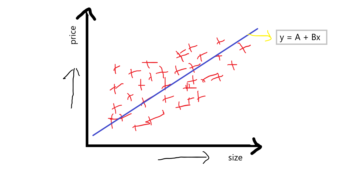
When we discuss this equation, in which the intersection basically indicates when the price of the house is 0 then what will be the base price of the house, and the slope or coefficient indicates that with the unit it increases in size, then what will be the unit increases in slope.
However, How is it different compared to multiple linear regression?
Multiple linear regression
Multiple linear regression basically indicates that we will have many characteristics such as f1, f2, f3, f4, and our output function f5. If we take the same example we discussed earlier, suppose:
f1 is the size of the house.
f2 They are bad rooms in the house.
f3 is the town of the house.
f4 is the state of the house and,
f5 it is our exit characteristic which is the price of the house.
Now, you can see that multiple standalone features have a huge impact on the price of the house too, price may vary from feature to feature. When we talk about multiple linear regression, then the simple linear regression equation y = A + Bx turns into something like:
equation: y = A + B1X1+ B2X2+ B3X3+ B4X4
“If we have a dependent function and several independent functions, we basically call it multiple linear regression. “
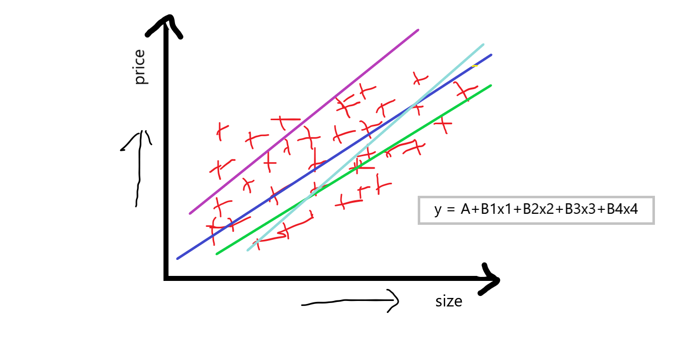
Now, our goal in using multiple linear regression is that we have to calculate A what is an intersection, Y B1 B2 B3 B4 what are the slopes or coefficients referring to this independent characteristic, which basically indicates that if we increase the value of X1 by 1 drive then B1 says how much value will affect the price of the house, and this was similar with respect to other B2 B3 B4
Then, this is a short theoretical description of multiple linear regression. We will now use the scikit learn linear regression library to solve the multiple linear regression problem.
Data set
Now, we apply multiple linear regression on the 50_startups data set, you can click here to download the dataset.
Read data set
Most of the dataset is in a CSV file, to read this file we use the pandas library:
df = pd.read_csv('50_Startups.csv')
df
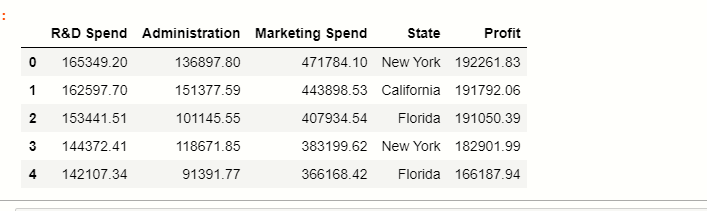
Here you can see what there is 5 columns in the dataset where the condition stores categorical data points and the rest are numeric characteristics.
Now, we have to classify independent and dependent characteristics:
Independent and dependent variables
There is a total of 5 characteristics in the data set, in which basically profits are our dependent characteristic, and the rest of them are our independent features:
#separate the other attributes from the predicting attribute
x = df.drop('Profit',axis=1)
#separte the predicting attribute into Y for model training
y = ['profit']
Management of categorical variables
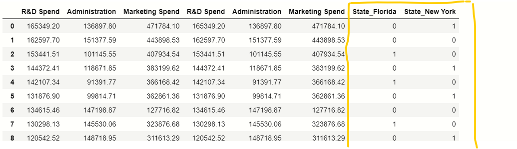
In our data set, there is a categorical column Condition, we have to handle these categorical values present inside this column for that we will use pandas get_dummies () function:
# handle variableIn statistics and mathematics, a "variable" is a symbol that represents a value that can change or vary. There are different types of variables, and qualitative, that describe non-numerical characteristics, and quantitative, representing numerical quantities. Variables are fundamental in experiments and studies, since they allow the analysis of relationships and patterns between different elements, facilitating the understanding of complex phenomena.... Categorical
estados = pd.get_dummies (x, drop_first = True)
# removing extra column
x = x.drop ('State', axis = 1)
# concatenation of independent variables and new cateoric variable.
x = pd.concat ([x,states], axis = 1)
X
Data division
Now, tenemos que dividir los datos en partes de trainingTraining is a systematic process designed to improve skills, physical knowledge or abilities. It is applied in various areas, like sport, Education and professional development. An effective training program includes goal planning, regular practice and evaluation of progress. Adaptation to individual needs and motivation are key factors in achieving successful and sustainable results in any discipline.... y prueba para las que usamos scikit-learn train_test_split () function.
# importing train_test_split from sklearn
from sklearn.model_selection import train_test_split
# splitting the data
x_train, x_test, y_train, y_test = train_test_split(x, Y, test_size = 0.2, random_state = 42)
Applying model
Now, we apply the linear regression model to our training data, first, we have to import linear regression from scikit-learn library, there is no other library to implement multiple linear regression, we do it only with linear regression.
# importing module
from sklearn.linear_model import LinearRegression
# creating an object of LinearRegression class
LR = LinearRegression()
# fitting the training data
LR.fit(x_train,y_train)
Finally, if we run this, then our model will be ready, now we have data from x_test, We use this data for the prediction of profit.
y_prediction =  LR.predict(x_test)
y_prediction

Now, we have to compare the y_prediction values with the original values because we have to calculate the precision of our model, which was implemented by a concept called r2_score. let's briefly discuss r2_score:
r2_score: –
It is a function within sklearn. metrics module, where the value of r2_score varies between 0 Y 100 percent, we can say that it is closely related to MSE.
r2 is basically calculated by the formula given below:
formula: r2 = 1 – (SSres / SSto mean )
now, when I Say SSres namely, is the sum of the residuals and SSto mean refers to the sum of means.
where,
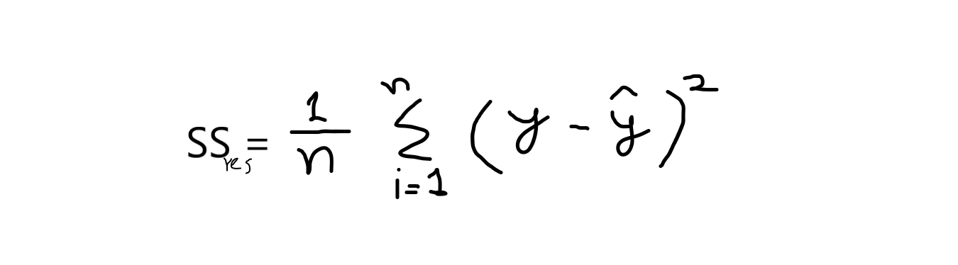
Y = original values
and ^ = predicted values. Y,
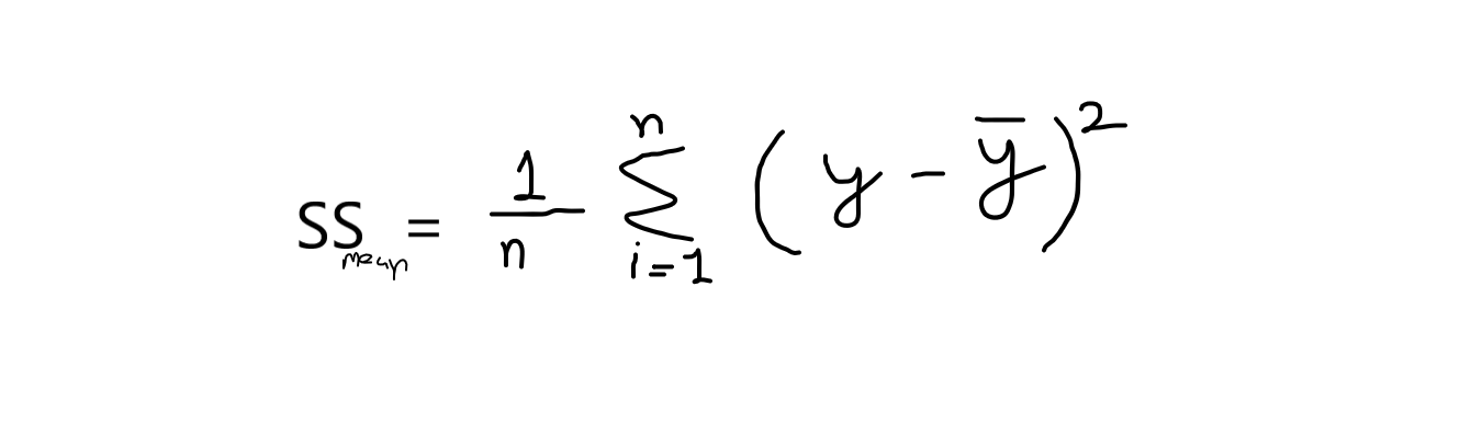
If we take the calculation of this equation, then we have to know that the value of the sum of the means is always greater than the sum of the residuals. If this condition is met, so our model is good for predictions. Their values range from 0,0 Y 1.
“The proportion of the variance in the dependent variable that is predictable from the (s) variable (s) Independent”.
The best possible score is 1.0 and it can be negative because the model can be arbitrarily worse. A constant model that always predicts the expected value of y, regardless of input characteristics, would get an R2 score of 0.0.
# importing r2_score module
de sklearn.metrics importar r2_score
de sklearn.metrics importar mean_squared_error
# predict accuracy score
score = r2_score (y_test, y_prediction)
print (‘r2 socre is’, punctuation)
print (‘mean_sqrd_error is ==’, mean_squared_error (y_test, y_prediction))
print (‘root_mean_squared error of is ==’, np.sqrt (mean_squared_error (y_test, y_prediction)))

You can see that the precision score is higher than 0,8, which means that we can use this model to solve multiple linear regressions, and also the root mean square error rate is also low.
Final notes
Hello there, data scientists 😎 above we took a detailed discussion on multiple linear regression, and the example we use is the perfect multiple linear regression example. Hope you now understand multiple linear regression better.
I hope you enjoyed this!
You can connect me on LinkedIn: www.linkedin.com/in/mayur-badole-189221199
What's more, read my other articles: https://www.analyticsvidhya.com/blog/author/mayurbadole2407/
Thanks.





