Multivariate time series | Vector automatic regression (WHERE)

Introduction

Time is the most critical factor in deciding whether a business will go up or down. This is why we see sales in stores and ecommerce platforms aligning with festivals.. These companies analyze years of spending data to understand the best time to open doors and see an increase in consumer spending..

But, How can you, as a data scientist, perform this analysis? Do not worry, you don't need to build a time machine! Time series modeling is a powerful technique that acts as a gateway to understand and forecast trends and patterns.

But even a model of Time SeriesA time series is a set of data collected or measured at successive times, usually at regular time intervals. This type of analysis allows you to identify patterns, Trends and cycles in data over time. Its application is wide, covering areas such as economics, Meteorology and public health, facilitating prediction and decision-making based on historical information.... has different facets. Most of the examples we see on the web deal with univariate time series. Unfortunately, real world use cases don't work like this. There are multiple variables at play, and handling them all at the same time is where a data scientist will gain his courage.

In this article, we will understand what a multivariate time series is and how to deal with it. We will also take a case study and implement it in Python to give you a practical understanding of the topic..

Table of Contents

1. Univariate versus multivariate time series
   1. Univariate time series
   2. Multivariate time series
2. Management of a multivariate time series: vector automatic regression (WHERE)
3. Why do we need VAR?
4. Stationarity in a multivariate time series
5. Train validation division
6. Python implementation

1. Univariate versus multivariate time series

This article assumes some familiarity with univariate time series, its properties and the various techniques used for prediction. Since this article will focus on multivariate time series, I suggest you review the following articles which serve as a good introduction to univariate time series:

But I'll give you a quick overview of what a univariate time series is., before going into the details of a multivariate time series. Let's look at them one by one to understand the difference.

1.1 Univariate time series

A univariate time series, as its name suggests, is a series with a single variableIn statistics and mathematics, a "variable" is a symbol that represents a value that can change or vary. There are different types of variables, and qualitative, that describe non-numerical characteristics, and quantitative, representing numerical quantities. Variables are fundamental in experiments and studies, since they allow the analysis of relationships and patterns between different elements, facilitating the understanding of complex phenomena.... time dependent.

For instance, have a look at the sample data set below consisting of the temperature values (hourly), during the last 2 years. Here, temperature is the dependent variable (time dependent).

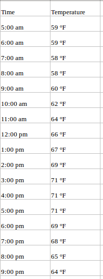
If we are asked to forecast the temperature for the next few days, we will look at the past values ​​and try to measure and extract a pattern. We would notice that the temperature is lower in the morning and at night, while it peaks in the afternoon. What's more, if you have data from the last years, you will notice that it is colder during the months of November to January, while it is comparatively hotter in April to June.

Such observations will help us predict future values.. Did you notice that we use only one variable (the temperature of the last 2 years)? Therefore, this is called Analysis / Univariate Time Series Forecast.

1.2 Multivariate time series (MTS)

A multivariate time series has more than one time-dependent variable. Each variable depends not only on its past values, it also has some dependence on other variables. This dependency is used to forecast future values. Sounds complicated? Let me explain.

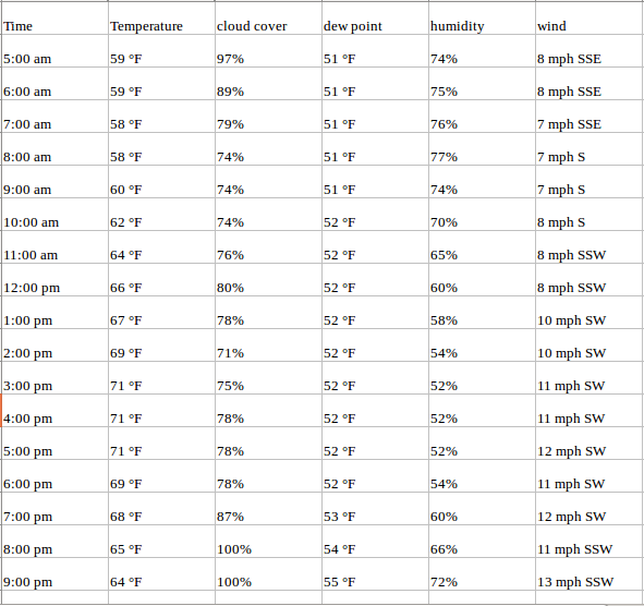
Consider the example above. Now suppose that our data set includes the percentage of perspiration, dew point, wind speed, the percentage of cloud cover, etc. together with the temperature value of the last two years. In this case, multiple variables must be considered to optimally predict temperature. A series like this would fall into the category of multivariate time series.. Below is an illustration of this:

Now that we understand what a multivariate time series looks like, let's understand how we can use it to build a forecast.

2. Management of a multivariate time series – WHERE

In this section, I will introduce you to one of the most used methods for multivariate time series forecasting: Vector automatic regression (WHERE).

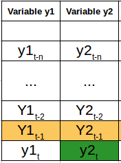
In a VAR model, each variable is a linear function of the past values ​​of itself and the past values ​​of all other variables. To explain this in a better way, I am going to use a simple visual example:

We have two variables, y1 e y2. We need to forecast the value of these two variables at time t, from the data given for the n passed values. To simplify, I have taken the delay value to be 1.

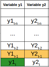
To calculate y1

Here,

• a1 and a2 are the constant terms,
• w11, w12, w21 and w22 are the coefficients,
• e1 and e2 are the error terms

These equations are similar to the equation of an AR process. Since the AR process is used for univariate time series data, future values ​​are linear combinations of your own past values ​​only. Consider the AR process (1):

Y

In this case, we have only one variable – Y, a constant term – a, an error term – e, and a coefficient – w. To accommodate the multiple variable terms in each equation for VAR, we will use vectors. We can write the equations (1) Y (2) as follows:

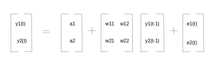
The two variables are y1 and y2, followed by a constant, a coefficient metric, a delay value and an error metric. This is the vector equation for a VAR process (1). For a VAR process (2), another vector term will be added for time (t-2) to the equation to generalize for lags:

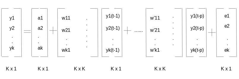
The above equation represents a VAR process (p) with variables y1, y2… yk. The same can be written as:

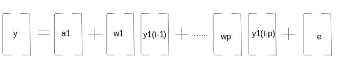
The term ε_t in the equation represents the multivariate vector white noise. For a multivariate time series, e_t must be a continuous random vector that satisfies the following conditions:

1. E (e_t) = 0
   The expected value for the error vector is 0
2. E (e_t1, e_t2‘) = σ₁₂
   Expected value of ε_t y ε_t‘Is the standard deviation of the series

3. Why do we need VAR?

Remember the example of forecasting temperate temperatures we saw earlier. It can be argued that it will be treated as a multiple univariate series. We can solve it using simple univariate forecasting methods like AR. Since the goal is to predict the temperature, we can just remove the other variables (except temperature) and fit a model to the remaining univariate series.

Another simple idea is to forecast the values ​​of each series individually using the techniques we already know.. This would make the job extremely easy!! Then, Why should I learn another forecasting technique? Isn't this topic complicated enough already?

From the above equations (1) Y (2), it is clear that each variable is using the past values ​​of each variable to make the predictions. Unlike AR, VAR is able to understand and use the relationship between several variables.. This is useful for describing the dynamic behavior of the data and also provides better forecasting results.. What's more, implementing VAR is as simple as using any other univariate technique (what you will see in the last section).

4. Stationarity of a multivariate time series

We know from the study of the univariate concept that a stationary time series will give us, In most cases, a better set of predictions. If you are not familiar with the concept of stationarity, read this article first: A gentle introduction to handling non-stationary time series.

To sum up, for a given univariate time series:

Y

The series is said to be stationary if the value of | c | <1. Now, remember the equation of our VAR process:

Note: I is the identity matrix.

Represent the equation in terms of Delay operators, have:

Taking all the terms and

The coefficient of y

#import required packages
import pandas as pd
import matplotlib.pyplot as plt
%matplotlib inline

#read the data
df = pd.read_csv("AirQualityUCI.csv", parse_dates=[['Date', 'Time']])

#check the dtypes
df.dtypes

Date_Time        object
CO(GT)            int64
PT08.S1(CO)       int64
NMHC(GT)          int64
C6H6(GT)          int64
PT08.S2(NMHC)     int64
NOx(GT)           int64
PT08.S3(NOx)      int64
NO2(GT)           int64
PT08.S4(NO2)      int64
PT08.S5(O3)       int64
T                 int64
RH                int64
AH                int64
dtype: object

df['Date_Time'] = pd.to_datetime(df.Date_Time , format="%d/%m/%Y %H.%M.%S")
data = df.drop(['Date_Time'], axis=1)
data.index = df.Date_Time

#missing value treatment
cols = data.columns
for j in cols:
    for i in range(0,len(data)):
       if data[j][i] == -200:
           data[j][i] = data[j][i-1]

#checking stationarity
from statsmodels.tsa.vector_ar.vecm import coint_johansen
#since the test works for only 12 variables, I have randomly dropped
#in the next iteration, I would drop another and check the eigenvalues
johan_test_temp = data.drop([ 'CO'(GT)'], axis=1)
coint_johansen(johan_test_temp,-1,1).own

array([ 0.17806667,  0.1552133 ,  0.1274826 ,  0.12277888,  0.09554265,
        0.08383711,  0.07246919,  0.06337852,  0.04051374,  0.02652395,
        0.01467492,  0.00051835])

#creating the train and validation set
train = data[:int(0.8*(len(data)))]
valid = data[int(0.8*(len(data))):]

#fit the model
from statsmodels.tsa.vector_ar.var_model import VAR

model = VAR(endog = train)
model_fit = model.fit()

# make prediction on validation
prediction = model_fit.forecast(model_fit.y, steps = len(valid))

#converting predictions to dataframe
pred = pd.DataFrame(index=range(0,len(prediction)),columns=[cols])
for j in range(0,13):
    for i in range(0, len(prediction)):
       pred.iloc[i][j] = prediction[i][j]

#check rmse
for i in cols:
    print('rmse value for', i, 'is' : ', sqrt(mean_squared_error(pred[i], valid[i])))

rmse value for CO(GT) is :  1.4200393103392812
rmse value for PT08.S1(CO) is :  303.3909208229375
rmse value for NMHC(GT) is :  204.0662895081472
rmse value for C6H6(GT) is :  28.153391799471244
rmse value for PT08.S2(NMHC) is :  6.538063846286176
rmse value for NOx(GT) is :  265.04913993413805
rmse value for PT08.S3(NOx) is :  250.7673347152554
rmse value for NO2(GT) is :  238.92642219826683
rmse value for PT08.S4(NO2) is :  247.50612831072633
rmse value for PT08.S5(O3) is :  392.3129907890131
rmse value for T is :  383.1344361254454
rmse value for RH is :  506.5847387424092
rmse value for AH is :  8.139735443605728

#make final predictions
model = VAR(even = data)
model_fit = model.fit()
yhat = model_fit.forecast(model_fit.y, steps=1)
print(yhat)