Simple linear regression in Python

Introduction

Hello everyone for this handy introduction to machine learning using simple linear regression.. Then let's get started:

Then, let's get acquainted with the terms that will be used:

Machine learning (ML): ML is an Artificial Intelligence application (HE) which gives systems the ability to automatically learn and improve from experience without being explicitly programmed. ML focuses on the development of computer programs that can access data and use it to learn by themselves.

Data set: A collection of related information sets that is made up of separate elements but that can be manipulated as a unit by a computer.

Data visualization: It is a representation of data or information in a graph, chart or other visual formats that are useful for analysis, like predictive analytics, which can serve as a useful visualization to present.

Data cleansing: It is the process of correcting or removing incorrect data, corrupt, incorrectly formatted, duplicates or incomplete within a data set.

Supervised learningSupervised learning is a machine learning approach where a model is trained using a set of labeled data. Each input in the dataset is associated with a known output, allowing the model to learn to predict outcomes for new inputs. This method is widely used in applications such as image classification, speech recognition and trend prediction, highlighting its importance in...: The model is trained using 'tagged data'. Se dice que los conjuntos de datos contienen etiquetas que contienen parametersThe "parameters" are variables or criteria that are used to define, measure or evaluate a phenomenon or system. In various fields such as statistics, Computer Science and Scientific Research, Parameters are critical to establishing norms and standards that guide data analysis and interpretation. Their proper selection and handling are crucial to obtain accurate and relevant results in any study or project.... de entrada y salida. To simplify: 'The data is already tagged with the correct answer'.

Simple linear regression: Es un Modelo de Regresión que estima la relación entre la variableIn statistics and mathematics, a "variable" is a symbol that represents a value that can change or vary. There are different types of variables, and qualitative, that describe non-numerical characteristics, and quantitative, representing numerical quantities. Variables are fundamental in experiments and studies, since they allow the analysis of relationships and patterns between different elements, facilitating the understanding of complex phenomena.... independiente y la variable dependiente usando una línea recta [y = mx + c], where both variables must be quantitative.

Models: The results are obtained using algorithms and are composed of data from the model and a prediction algorithm..

Model of trainingTraining is a systematic process designed to improve skills, physical knowledge or abilities. It is applied in various areas, like sport, Education and professional development. An effective training program includes goal planning, regular practice and evaluation of progress. Adaptation to individual needs and motivation are key factors in achieving successful and sustainable results in any discipline....: In supervised learning, an ML algorithm creates a model by examining many examples and trying to find a model that minimizes loss and improves prediction accuracy.

These are the few terms that are used in this article and with which to become familiar. Now let's start with the analysis and prediction of the model. In this tutorial, I will use supervised data and simple linear regression for analysis and prediction. The ultimate goal is to predict a person's height and provide their age using the trained model as accurately as possible using the available data.. I have used the universal favorite programming language for ML, namely. Piton to build and train the ML model and the Google Colab environment.

The steps involved are:

1. Dataset import.

2. Data visualization

3. Data cleansing

4. Build the model and train it

5.Make predictions on invisible data

———————————————————————————————————————————————— ——————————

1. Dataset import:

The first and most important thing to do is import the dataset. We have several websites that have these data sets to be used by anyone. Similarly, let's start how to import the dataset that we are going to use in this tutorial.

This single line of code helps us get the data used for the tutorial directly from the URL.

Data set <- Click on the link to get the dataset which is the URL mentioned above.

2. Data visualization:

In this step, after importing the data and mounting it with Colab, let's get an overview of the dataset by importing a module called pandas. Since the data set we have has an extension of .pkl, we just see it by the function available in the pandas library.

We import the library to read the data set and store it in a variable called raw_data. Then we show the content of raw_data which is in tabulated format.

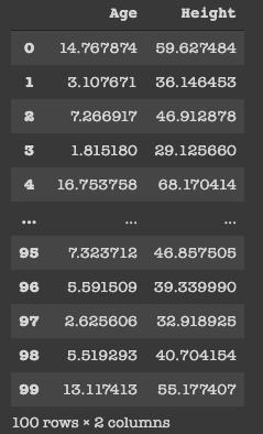
We can see the data that we have and contains only 2 columns, namely, Age (in years) and Height (in inches) Y 100 rows, which is actually the representation of a person.

This single line of code has a huge impact on the way we look at the dataset. We only had a numeric view of the dataset, but now we can run this cell to get a histogram view of the dataset, which is very useful. Represents the data present in the individual columns as individual charts.

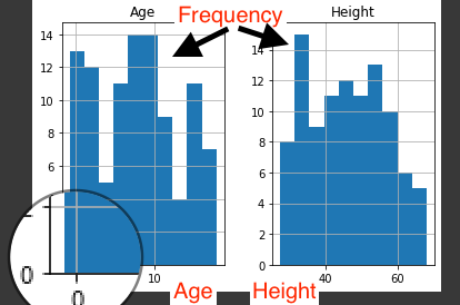
The Y axis in both graphs refers to frequency and the X axis represents Age and Height respectively..

3. Data cleansing:

We have to build the model using valid data sets and clean the unaccountable data. In the picture above, we can know that there are some entries that have an age less than zero, which doesn't make sense. Therefore, we need to clean that data to get more precision.

I use variable data_cleaned to store valid age values ​​and display them to the user.

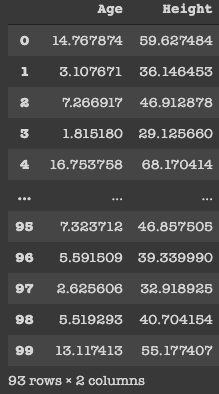
Initially, we had 100 rows, but after doing data cleaning, it is quite clear that there are seven rows that had an age <0 and we have removed them. As a professional, we are not supposed to delete the data, since we are reducing them and, Thus, the accuracy of our model is reduced. To keep it simple, I just deleted them.

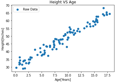
Visualize clean data: now i have used the clean data and visualized it as a graph.

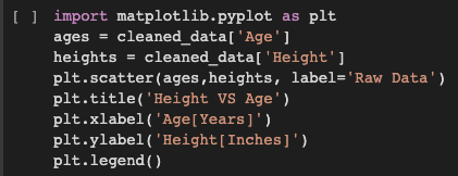
To plot python graphics, I import the matplotlib.pyplot library. I represent the age on the X axis and the height on the Y axis. The points on the graph refer to the raw data.

4. Build the model and train it:

This is where the ML algorithm comes in., namely, simple linear regression.

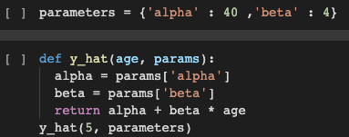
I used a dictionary called parameters which has alfa Y beta as key with 40 Y 4 as values ​​respectively. I have also defined a function y_hat which takes age and parameters as parameters. This function uses the basic equation in a straight line and returns y, namely, height as in our case. If we pass the required parameters and execute the function, we find that the height we get for the age as input does not match. Therefore, we use the below mentioned function to make the model rain.

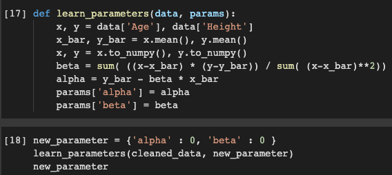
This is where we use a method to find the correct alpha and beta. The function learn_parameters you accept data_cleaned and a dummy dictionary new_parameter which can have any value for alpha and beta. Then, when we pass them as arguments to the parameters and the function executes, we can get the correct value of alpha and beta which is close to 30 Y 2 respectively and replace the old values ​​with the new ones.

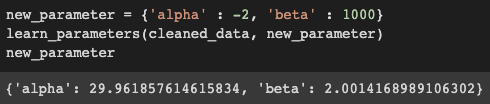
We have accurately found the alpha and beta values, and our next goal is to train the data. But let me the untrained predicted values ​​how accurate they are.

I use a list called spatial_ages which has values ​​of 0 a 18 (final – 1). Then another list called spaced_untrained_predictions which has the predicted values ​​for the height uses the y_hat function defined above to predict it. These values ​​are plotted on a graph and displayed.

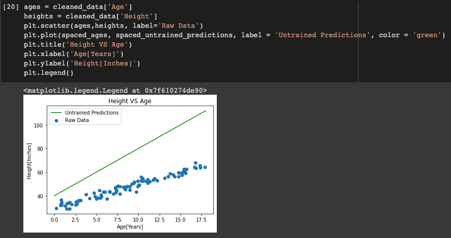
The green line shows that the spaced_untrained_predictions have deviated greatly from the actual values ​​and the accuracy is very poor. Therefore, it is necessary to increase the precision for which we must train the data.

So instead of using parameters we use new_parameters since it contains the exact value of alfa Y beta and stores it in a list called spaced_trained_predictions. Then, when we plot a graph for this, we can see a visible difference and the accuracy has increased a lot. Therefore, we have successfully built and trained the model. Proof of this are the values ​​of spaced_trained_predictions and the graph.

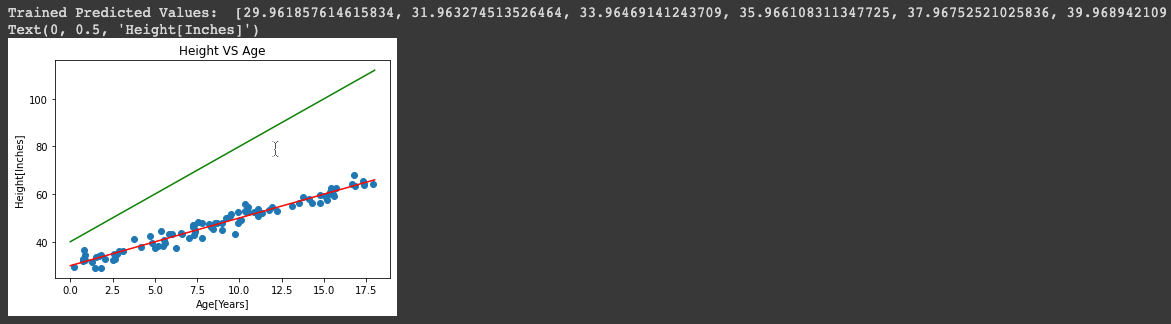
The Greenline refers to the values ​​of spaced_untrained_predictions and Redline refers to the values ​​of spaced_trained_predictions.

5.Make predictions on invisible data:

With the help of this trained model, now we can make accurate predictions.

Then, we can see that for any given age we find the possible height in inches. Finally, we have trained the model successfully and with the utmost precision, which is the end goal of this tutorial.

As reference, I have pasted the Link to notebook you play with him. I hope to connect through LinkedIn too and share your valuable comments. Stay tuned for more blogs of this type😊.

Related