SQL Techniques | Data analysis using SQL

Overview

• SQL is a must-have language for anyone in data science or analytics.
• Here there is 8 Ingenious SQL techniques for data analysis that analytics and data science professionals will love to work with

Introduction

SQL is a key gear in the arsenal of a data science professional. I speak from experience: you just can't hope to build a successful career in data science or analytics if you haven't learned SQL yet.

And why is SQL so important?

As we move into a new decade, the speed at which we produce and consume data is skyrocketing day by day. To make smart data-driven decisions, organizations around the world are hiring data professionals such as business analysts and data scientists to extract and unearth insights from the vast trove of data.

And one of the most important tools needed for this is, I guess it, ¡SQL!

The structured query language (SQL) has been around for decades. It is a programming language used to manage data stored in relational databases. SQL is used by most large companies around the world. A data analyst can use SQL to access, read, manipulate and analyze data stored in a database and generate useful information to drive an informed decision-making process.

In this article, I will discuss 8 techniques / SQL queries that will prepare you for any advanced data analysis problems. Please note that this article assumes a very basic understanding of SQL.

I would suggest checking out the courses below if you are new to SQL and / or business analysis:

Table of Contents

1. First let's understand the dataset
2. SQL Technique n. ° 1: count rows and elements
3. SQL Technique n. ° 2: aggregation functions
4. SQL technique # 3: Identification of extreme values
5. SQL Technique n. ° 4: data cut
6. SQL Technique n. ° 5: data limitation
7. SQL Technique n. ° 6: data classification
8. SQL Technique n. ° 7: filter patterns
9. SQL Technique n. ° 8: clusters, data accumulation and filtering in groups

First let's understand the dataset

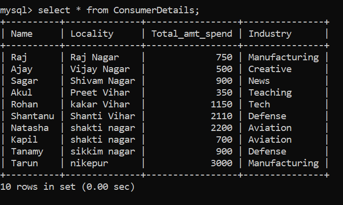
What is the best way to learn to analyze data? Doing it side by side on a data set!! For this purpose, I have created a dummy dataset of a retail store. The customer data table is represented by ConsumerDetails.

Our dataset consists of the following columns:

• Name – The consumer's name
• Location – The customer's location
• Total_amt_spend – The total amount of money spent by the consumer in the store.
• Industry – It means the industry to which the consumer belongs

Note: – I will use MySQL 5.7 to advance in the article. You can download it from here – Descargas de My SQL 5.7.

SQL Technique n. ° 1: row and item count

We will start our analysis with the simplest query, namely, counting the number of rows in our table. We will do this using the function – COUNT ().

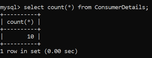
Excellent! Now we know the number of rows in our table, What is it 10. It may seem fun to use this function on a small set of test data, But it can go a long way when your ranks number in the millions!!

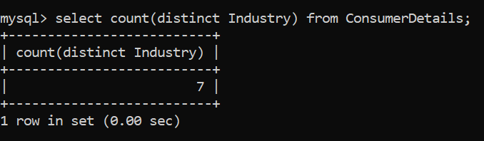
Many times, our data table is full of duplicate values. To achieve the unique value, we use the DISTINCT function.

In our data set, How can we find the unique industries that customers belong to?

You guessed it right. We can do this using the DISTINCT function.

You can even count the number of unique rows by using counting in conjunction with different. You can refer to the following query:

SQL technique # 2 – Aggregation functions

Aggregation functions are the basis of any type of data analysis. They give us an overview of the dataset. Some of the functions we will discuss are: SUM (), AVG () and STDDEV ().

We use the SUM() function to calculate the sum of the numeric column in a table.

Let's find out the sum of the amount spent by each of the clients:

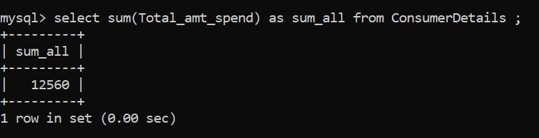
In the example above, sum_all is the variable in which the value of the sum is stored. The sum of the amount of money spent by consumers is Rs. 12.560.

To calculate the average of numeric columns, we use the AVG () function. Let's find average consumer spending for our retail store:

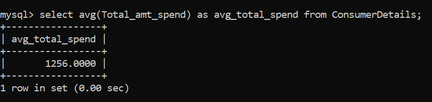
The average amount spent by customers in the retail store is Rs. 1256.

• Calculate the standard deviation

If you have looked at the dataset and then the average value of consumer spending, you will have noticed that something is missing. Average does not provide a complete picture, so let's look for another important metric: the standard deviation. The function is STDDEV ().

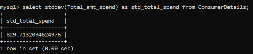
The standard deviation turns out to be 829,7, which means that there is a large disparity between consumer spending.

SQL technique # 3 – Identification of extreme values

The next type of analysis is to identify extreme values ​​that will help you better understand the data..

The maximum numerical value can be identified by the MAX function (). Let's see how to apply it:

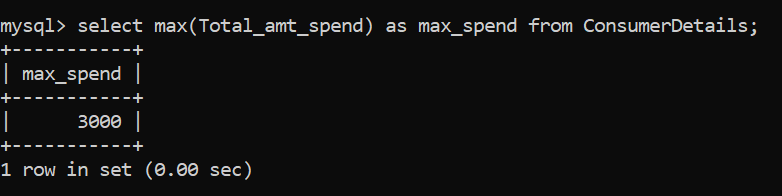
The maximum amount of money that the consumer spends in the retail store is Rs. 3000.

Similar to the max function, we have the MIN function () to identify the minimum numeric value in a given column:

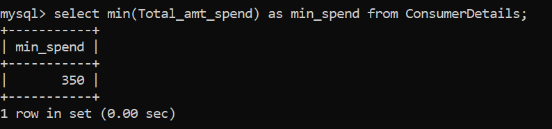
The minimum amount of money spent by the retail store consumer is Rs. 350.

SQL Technique n. ° 4: data cut

Now, let's focus on one of the most important parts of data analysis: divide the data. This section of the analysis will form the basis for advanced queries and help you to retrieve data based on some kind of condition.

• Let's say the retail store wants to find customers who come from a locality, specifically Shakti Nagar and Shanti Vihar. What will be the query for this?

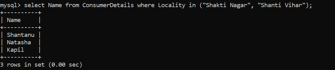
¡Genial, have 3 customers! We have used the WHERE clause to filter the data based on the condition that consumers should live in the locality: Shakti Nagar y Shanti Vihar. I did not use the OR condition here. Instead, I have used the IN operator which allows us to specify multiple values ​​in the WHERE clause.

• We need to find clients who live in specific locations (Shakti Nagar y Shanti Vihar) and spend an amount greater than Rs. 2000.

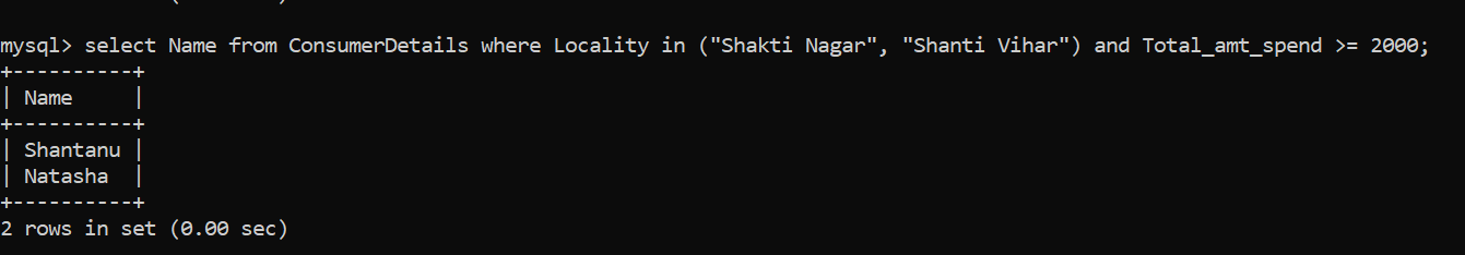
In our data set, only Shantanu and Natasha meet these conditions. How both conditions must be met, the AND condition is best suited here. Let's see another example to divide our data.

• This time, the retail store wants to win back all consumers who spend between Rs. 1000 y Rs. 2000 to drive special marketing offers. What will be the query for this?

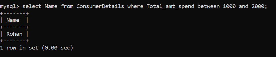
Another way to write the same statement would be:

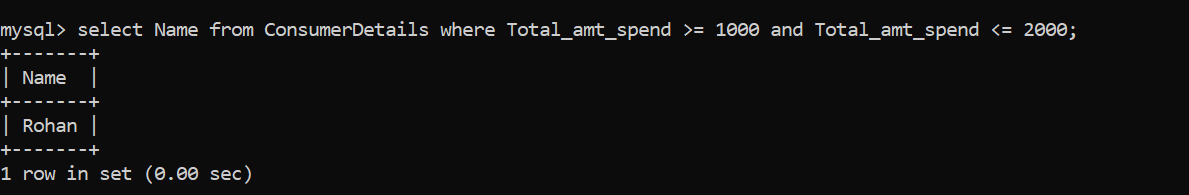
Only Rohan is clearing this criterion!!

Excellent! We have reached the middle of our journey. Let's build more on the knowledge we've gained so far.

SQL Technique n. ° 5: data limitation

Let's say we want to see the data table consisting of millions of records. We cannot use the SELECT statement directly as this would dump the entire table on our screen, which is cumbersome and computationally intensive. Instead, we can use the LIMIT clause:

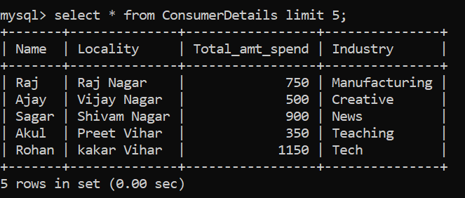
The above SQL command helps us to show the first 5 table rows.

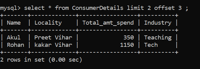
What will you do if you only want to select the fourth and fifth rows? We will use the OFFSET clause. The OFFSET clause will skip the specified number of rows. Let's see how it works:

SQL Technique n. ° 6: data classification

Sorting data helps us put our data in perspective. We can perform the classification process using the keyword – ORDER BY.

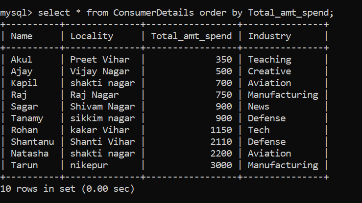
The keyword can be used to sort the data in ascending or descending order. The ORDER BY keyword sorts the data in ascending order by default.

Let's see an example in which we sort the data according to the Total_amt_spend column in ascending order:

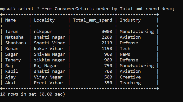
Impressive! To sort the dataset in descending order, we can follow the following command:

SQL technique # 7 – Filtering patterns

In the previous sections, we learned how to filter data based on one or more conditions. Here, we will learn how to filter the columns that match a specific pattern. To get on with this, we will first understand the LIKE operator and wildcard characters.

The LIKE operator is used in a WHERE clause to find a specific pattern in a column.

The wildcard character is used to substitute one or more characters in a string. These are used in conjunction with the LIKE operator. The two most common wildcard characters are:

• • %: It represents 0 or more characters
  • _ – Represents a single character

In our fictitious retail dataset, let's say we want all the localities that end with "Nagar". Take a moment to understand the problem statement and think about how we can solve it.

Let's try to solve the problem. We require all locations ending with “Nagar” and they can have any number of characters before this particular string. Therefore, we can make use of the wild card “%” before “Nagar”:

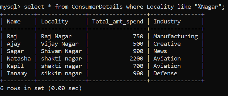
Impressive, have 6 localities that end with this name. Notice that we are using the LIKE operator to perform pattern matching.

Then, we will try to solve another problem based on patterns. We want the names of consumers whose second character has “a” in their respective names. Again, I suggest you take a moment to understand the problem and think of a logic to solve it.

Let's analyze the problem. Here, the second character must be “a”. The first character can be anything, so we substitute this letter for the wildcard "_". After the second character, there can be any number of characters, so we substitute those characters with the wildcard “%”. The final pattern match will look like this:

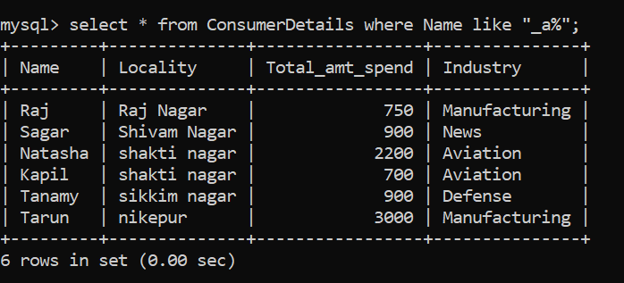
Have 6 people who satisfy this strange condition!

SQL Technique n. ° 8: clusters, data accumulation and filtering in groups

We have finally arrived at one of the most powerful analysis tools in SQL: the grouping of data that is done using the GROUP BY statement. The most useful application of this statement is to find the distribution of categorical variables. This is done using the GROUP BY statement in conjunction with aggregation functions like – COUNT, SUM, AVG, etc.

Let's try to understand this better by taking a statement of the problem. The retail store wants to find the number of customers corresponding to the industries to which it belongs:

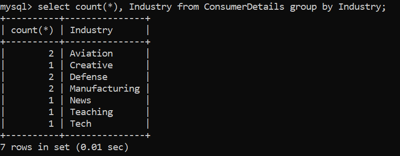
We observe that the count of clients belonging to the different industries is more or less the same. Then, Let's go ahead and find the sum of the expenses of the clients grouped by the industry to which they belong:

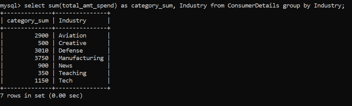
We can see that the maximum amount of money spent is by customers belonging to the Manufacturing industry. This seems a bit easy, truth? Let's step forward and make it more complicated.

Now, the retailer wants to find the industries whose Total amount is greater than 2500. To solve this problem, we will regroup the data by industry and then use the HAVING clause.

HAVING clause is like WHERE clause but only to filter grouped data. Remember, will always come after the GROUP BY statement.

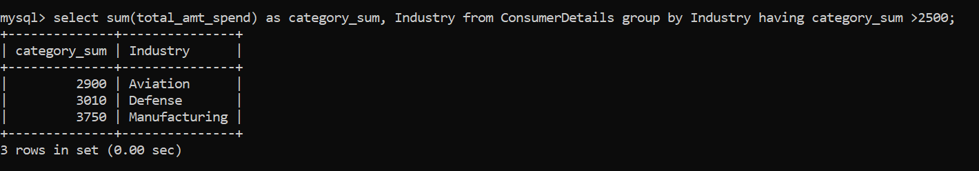
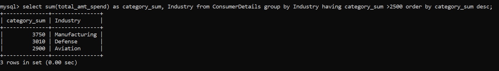
We have only 3 categories that satisfy the conditions: Aviation, Defending, Y Manufacturing. But to make it clearer, I will also add the ORDER BY keyword to make it more intuitive:

Final notes

I'm so glad you made it this far. These are the building blocks of all data analysis queries in SQL. You can also do advanced queries using these basics. In this article, i used mysql 5.7 to set the examples.

I really hope these SQL queries help you in your day to day when you are analyzing complex data. Have any of their tips and tricks for analyzing data in SQL? Let me know in the comments!!

Related