
This article was published as part of the Data Science Blogathon
“Generative Adversarial Networks is the most interesting idea in the last ten years in Machine Learning” – Yann LeCun
Introduction
mathematical understanding and practice of it, but before that, if you want to take a look at the basics of GAN, you can continue with the following link:
Most of the tech giants (like Google, Microsoft, Amazon, etc.) are working hard to apply GANs to practical use, some of these use cases are:
- Adobe: using GAN for your next-gen Photoshop.
- Google: using GAN for text generation.
- IBM: use of GAN for data augmentation (to generate synthetic images to train your classification models).
- Snap Chat / TikTok: to create multiple image filters (that you may have already seen).
- Disney: uso de GAN para súper resolutionThe "resolution" refers to the ability to make firm decisions and meet set goals. In personal and professional contexts, It involves defining clear goals and developing an action plan to achieve them. Resolution is critical to personal growth and success in various areas of life, as it allows you to overcome obstacles and keep your focus on what really matters.... (video quality improvement) for your movies.
Something that is special about GANs is that these companies depend on them for their future., Don't you think?
Then, What's stopping you from gaining the knowledge of this epic technology? I will answer you, any, you just need one advantage and this article would. Let's first discuss the math behind Generator and Discriminator.
Mathematical operation of the discriminator:
The sole purpose of the Discriminator is to classify real and fake images. For classification, utiliza una red neuronal convolucionalConvolutional Neural Networks (CNN) are a type of neural network architecture designed especially for data processing with a grid structure, as pictures. They use convolution layers to extract hierarchical features, which makes them especially effective in pattern recognition and classification tasks. Thanks to its ability to learn from large volumes of data, CNNs have revolutionized fields such as computer vision.. (CNN) traditional with a specific cost function. The Discriminator training process works as follows:
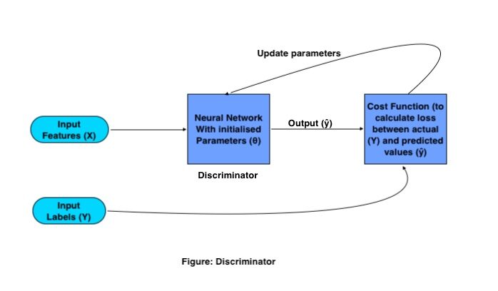
Where X and Y are input characteristics and labels respectively, the output is represented by (ŷ) and the parametersThe "parameters" are variables or criteria that are used to define, measure or evaluate a phenomenon or system. In various fields such as statistics, Computer Science and Scientific Research, Parameters are critical to establishing norms and standards that guide data analysis and interpretation. Their proper selection and handling are crucial to obtain accurate and relevant results in any study or project.... de red se representan con (θ).
Los GAN de trainingTraining is a systematic process designed to improve skills, physical knowledge or abilities. It is applied in various areas, like sport, Education and professional development. An effective training program includes goal planning, regular practice and evaluation of progress. Adaptation to individual needs and motivation are key factors in achieving successful and sustainable results in any discipline.... necesitan un conjunto de imágenes de entrenamiento y sus respectivas etiquetas, these images as an input feature go to CNN, with a set of initialized parameters. This CNN generates output by multiplying the weight matrix (W) with input characteristics (X) and adding a Bias (B) en ella y convirtiéndola en una matriz no lineal pasándola a una wake functionThe activation function is a key component in neural networks, since it determines the output of a neuron based on its input. Its main purpose is to introduce nonlinearities into the model, allowing you to learn complex patterns in data. There are various activation functions, like the sigmoid, ReLU and tanh, each with particular characteristics that affect the performance of the model in different applications.....
This output is known as predicted output., then the loss is calculated based on the weight parameters that are adjusted in the network to minimize the loss.
Mathematical operation of the generator:
The purpose of the Generator is to generate a false image from the given distribution (set of images), it does it with the following procedure:
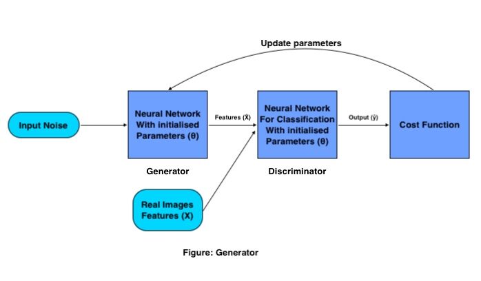
A set of input vectors is passed (random noise) through the red neuronalNeural networks are computational models inspired by the functioning of the human brain. They use structures known as artificial neurons to process and learn from data. These networks are fundamental in the field of artificial intelligence, enabling significant advancements in tasks such as image recognition, Natural Language Processing and Time Series Prediction, among others. Their ability to learn complex patterns makes them powerful tools.. del generador, which creates a whole new image by multiplying the generator weight matrix with the input noise.
This generated image works as input to the discriminator that is trained to classify fake and real images.. Then the loss is calculated for the generated images, based on what parameters are updated for the generator until we get good precision.
Once we are satisfied with the accuracy of the Generator, We save the Generator weights and eliminate the Discriminator from the network, and we use that weight matrix to generate more new images by passing it a different random noise matrix each time.
Binary Cross Entropy Loss for GAN:
To optimize GAN parameters, we need a cost function that tells the network how much it needs to improve simply by calculating the difference between the actual and predicted value. The Loss functionThe loss function is a fundamental tool in machine learning that quantifies the discrepancy between model predictions and actual values. Its goal is to guide the training process by minimizing this difference, thus allowing the model to learn more effectively. There are different types of loss functions, such as mean square error and cross-entropy, each one suitable for different tasks and... que se utiliza en las GAN se denomina entropía cruzada binaria y se representa como:

Where m is the batch size, Y(I) is the actual tag value, h is the predicted label value, x(I) is the input characteristic and θ represents the parameter.
Let's divide this cost function into subparts to better understand. The given formula is the combination of two terms where one is used when it is effective when the label is “0” and the other is important when the label is “1”. The first term is:
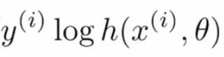
if the real value is “1” and the predicted value is “~ 0” in this case, since log (~ 0) tends to negative infinity or very high, and if the predicted value is also “~ 1”, then the log ( ~ 1) would be close to “0” or very less, so this term helps to calculate the loss for the label values “1”.

If the actual value is “0” and the predicted value is “~ 1”, then log (1- (~ 1)) would result in negative infinity or very high, and if the predicted value is “~ 0”, then the term would produce results "~ 0" or much less loss, so this term is used for the actual tag values "0".
Any of the loss terms would return negative values in case the prediction is wrong, the combination of these terms is called Entropy (logarithmic loss). But since it is negative, to make it greater than "1" we apply a negative sign (can be seen in the main formula), applying this negative sign is what does it Cross entropy (negative logarithmic loss).
Let's train the first GAN model:
We will create a GAN model that could generate handwritten digits from the MNIST data distribution using the PyTorch module.
First, let's import the required modules:
%matplotlib inline
import numpy as np
import torch
import matplotlib.pyplot as plt
Then we would read the data from the submodule provided by PyTorch called data sets.
# number of subprocesses to use for data loading
num_workers = 0
# how many samples per batch to load
batch_size = 64
# convert data to torch.FloatTensor
transform = transforms.ToTensor()
# get the training datasets
train_data = datasets.MNIST(root="data", train=True,
                                   download=True, transform=transform)
# prepare data loader
train_loader = torch.utils.data.DataLoader(train_data, batch_size=batch_size,
                                           num_workers=num_workers)
Visualize the data
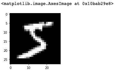
Since we would be creating our model in the PyTorch framework that uses tensors, we would be turning our data into torch tensioners. If you want to view the data, you can go ahead and use the following code snippet:
# obtain one batch of training images
dataiter = iter(train_loader)
images, labels = dataiter.next()
images = images.numpy()
# get one image from the batch
img = np.squeeze(images[0])
fig = plt.figure(figsize = (3,3))
ax = fig.add_subplot(111)
ax.imshow(img, cmap='gray')
Discriminated
Now is the time to define the Discriminator network, which is the combination of several layers of CNN.
import torch.nn as nn
import torch.nn.functional as F
class Discriminator(nn.Module):
    def __init__(self, input_size, hidden_dim, output_size):
        super(Discriminator, self).__init__()
        # define hidden linear layers
        self.fc1 = nn.Linear(input_size, hidden_dim*4)
        self.fc2 = nn.Linear(hidden_dim*4, hidden_dim*2)
        self.fc3 = nn.Linear(hidden_dim*2, hidden_dim)
        # final fully-connected layer
        self.fc4 = nn.Linear(hidden_dim, output_size)
        # dropout layer
        self.dropout = nn.Dropout(0.3)
    def forward(self, x):
        # flatten image
        x = x.view(-1, 28*28)
        # all hidden layers
        x = F.leaky_relu(self.fc1(x), 0.2) # (input, negative_slope=0.2)
        x = self.dropout(x)
        x = F.leaky_relu(self.fc2(x), 0.2)
        x = self.dropout(x)
        x = F.leaky_relu(self.fc3(x), 0.2)
        x = self.dropout(x)
        # final layer
        out = self.fc4(x)
        return out
The above code follows the traditional object-oriented Python architecture. fc1, fc2, fc3, fc3 are the fully connected layers. When we pass our input entities, goes through all these layers starting from fc1, At the end, we have an abandonment layer that is used to address the overfitting issue.
In the same code, you will see a function called forward (self, x), this function is the implementation of the actual forward propagation mechanism where each layer (fc1, fc2, fc3 and fc4) is followed by a trigger function (leaping_relu ) to convert the liner output to non-linear.
Generator Model
After that, we will verify the Generator segment of GAN:
class Generator(nn.Module):
    def __init__(self, input_size, hidden_dim, output_size):
        super(Generator, self).__init__()
        # define hidden linear layers
        self.fc1 = nn.Linear(input_size, hidden_dim)
        self.fc2 = nn.Linear(hidden_dim, hidden_dim*2)
        self.fc3 = nn.Linear(hidden_dim*2, hidden_dim*4)
        # final fully-connected layer
        self.fc4 = nn.Linear(hidden_dim*4, output_size)
        # dropout layer
        self.dropout = nn.Dropout(0.3)
    def forward(self, x):
        # all hidden layers
        x = F.leaky_relu(self.fc1(x), 0.2) # (input, negative_slope=0.2)
        x = self.dropout(x)
        x = F.leaky_relu(self.fc2(x), 0.2)
        x = self.dropout(x)
        x = F.leaky_relu(self.fc3(x), 0.2)
        x = self.dropout(x)
        # final layer with tanh applied
        out = F.tanh(self.fc4(x))
        return out
The generator network is also built from the fully connected layers, las funciones de activación de resumeThe ReLU activation function (Rectified Linear Unit) It is widely used in neural networks due to its simplicity and effectiveness. Defined as ( f(x) = max(0, x) ), ReLU allows neurons to fire only when the input is positive, which helps mitigate the problem of gradient fading. Its use has been shown to improve performance in various deep learning tasks, making ReLU an option... con fugas y la deserción. The only thing that makes it different from Discriminator is that it outputs depending on the output_size parameter (what is the size of the image to be generated).
Hyperparameter tuning
The hyperparameters that we are going to use to train the GANs are:
# Discriminator hyperparams
# Size of input image to discriminator (28*28)
input_size = 784
# Size of discriminator output (real or fake)
d_output_size = 1
# Size of last hidden layer in the discriminator
d_hidden_size = 32
# Generator hyperparams
# Size of latent vector to give to generator
z_size = 100
# Size of discriminator output (generated image)
g_output_size = 784
# Size of first hidden layer in the generator
g_hidden_size = 32
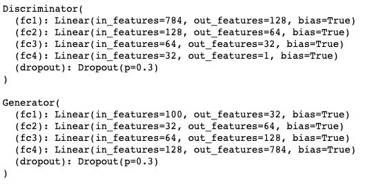
Create an instance of the models
And finally, the entire network would look like this:
# instantiate discriminator and generator
D = Discriminator(input_size, d_hidden_size, d_output_size)
G = Generator(z_size, g_hidden_size, g_output_size)
# check that they are as you expect
print(D)
print( )
print(G)
Calculate losses
We have defined the Generator and the Discriminator now it is time to define your losses so that those networks improve over time. For the GAN we would have two real losses of loss function and false loss that would be defined like this:
# Calculate losses
def real_loss(D_out, smooth=False):
    batch_size = D_out.size(0)
    # label smoothing
    if smooth:
        # smooth, real labels = 0.9
        labels = torch.ones(batch_size)*0.9
    else:
        labels = torch.ones(batch_size) # real labels = 1
    # numerically stable loss
    criterion = nn.BCEWithLogitsLoss()
    # calculate loss
    loss = criterion(D_out.squeeze(), labels)
    return loss
def fake_loss(D_out):
    batch_size = D_out.size(0)
    labels = torch.zeros(batch_size) # fake labels = 0
    criterion = nn.BCEWithLogitsLoss()
    # calculate loss
    loss = criterion(D_out.squeeze(), labels)
    return loss
Optimizers
Once the losses are defined, we would choose a suitable optimizer for training:
import torch.optim as optim
# Optimizers
lr = 0.002
# Create optimizers for the discriminator and generator
d_optimizer = optim.Adam(D.parameters(), lr)
g_optimizer = optim.Adam(G.parameters(), lr)
Model training
Since we have defined Generator and Discriminator both the networks, its loss functions as optimizers, now we would use the times and other characteristics to train the whole network.
import pickle as pkl
# training hyperparams
num_epochs = 100
# keep track of loss and generated, "fake" samples
samples = []
losses = []
print_every = 400
# Get some fixed data for sampling. These are images that are held
# constant throughout training, and allow us to inspect the model's performance
sample_size=16
fixed_z = np.random.uniform(-1, 1, size=(sample_size, z_size))
fixed_z = torch.from_numpy(fixed_z).float()
# train the network
D.train()
G.train()
for epoch in range(num_epochs):
    for batch_i, (real_images, _) in enumerate(train_loader):
        batch_size = real_images.size(0)
        ## Important rescaling step ##
        real_images = real_images*2 - 1  # rescale input images from [0,1) to [-1, 1)
        # ============================================
        #            TRAIN THE DISCRIMINATOR
        # ============================================
        d_optimizer.zero_grad()
        # 1. Train with real images
        # Compute the discriminator losses on real images
        # smooth the real labels
        D_real = D(real_images)
        d_real_loss = real_loss(D_real, smooth=True)
        # 2. Train with fake images
        # Generate fake images
        # gradients don't have to flow during this step
        with torch.no_grad():
            z = np.random.uniform(-1, 1, size=(batch_size, z_size))
            z = torch.from_numpy(With).float()
            fake_images = G(With)
        # Compute the discriminator losses on fake images
        D_fake = D(fake_images)
        d_fake_loss = fake_loss(D_fake)
        # add up loss and perform backprop
        d_loss = d_real_loss + d_fake_loss
        d_loss.backward()
        d_optimizer.step()
        # =========================================
        #            TRAIN THE GENERATOR
        # =========================================
        g_optimizer.zero_grad()
        # 1. Train with fake images and flipped labels
        # Generate fake images
        z = np.random.uniform(-1, 1, size=(batch_size, z_size))
        z = torch.from_numpy(With).float()
        fake_images = G(With)
        # Compute the discriminator losses on fake images
        # using flipped labels!
        D_fake = D(fake_images)
        g_loss = real_loss(D_fake) # use real loss to flip labels
        # perform backprop
        g_loss.backward()
        g_optimizer.step()
        # Print some loss stats
        if batch_i % print_every == 0:
            # print discriminator and generator loss
            print('Epoch' [{:5d}/{:5d}] | d_loss: {:6.4f} | g_loss: {:6.4f}.format(
                    epoch+1, num_epochs, d_loss.item(), g_loss.item()))
    ## AFTER EACH EPOCH##
    # append discriminator loss and generator loss
    losses.append((d_loss.item(), g_loss.item()))
    # generate and save sample, fake images
    G.eval() # eval mode for generating samples
    samples_z = G(fixed_z)
    samples.append(samples_z)
    G.train() # back to train mode
# Save training generator samples
with open('train_samples.pkl', 'wb') as f:
    pkl.dump(samples, f)
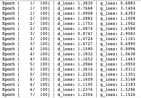
Once you run the above code snippet, the training process would start like this:
Generate images
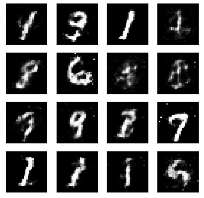
Finally, when the model is trained, you can use the trained generator to produce the new handwritten images.
# randomly generated, new latent vectors
sample_size=16
rand_z = np.random.uniform(-1, 1, size=(sample_size, z_size))
rand_z = torch.from_numpy(rand_z).float()
G.eval() # eval mode
# generated samples
rand_images = G(rand_z)
# 0 indicates the first set of samples in the passed in list
# and we only have one batch of samples, here
view_samples(0, [rand_images])
The output generated with the following code would like something like this:
Then, now that you have your own trained GAN model, you can use this model to train you on a different set of images, to produce new invisible images.
References:
1. Deep learningDeep learning, A subdiscipline of artificial intelligence, relies on artificial neural networks to analyze and process large volumes of data. This technique allows machines to learn patterns and perform complex tasks, such as speech recognition and computer vision. Its ability to continuously improve as more data is provided to it makes it a key tool in various industries, from health... de Udacity: https://www.udacity.com/
2. Deep learning artificial intelligence: https://www.deeplearning.ai/
Thanks for reading this article. If you have learned something new, feel free to comment! See you next time! !!! ❤️
The media shown in this article is not the property of DataPeaker and is used at the author's discretion.





