
Introduction
Today, one of the trendy social media platforms is .... guess what? A single WhatsApp😅. It is one of the favorite social media platforms among all of us due to its attractive features. Has more than 2 one billion users worldwide and “According to a survey, an average user spends more than 195 minutes a week on WhatsApp”. How terrible is the above statement. Drop all these things and let's understand what the WhatsApp analyzer really means.
WhatsApp Analyzer means that we are analyzing our WhatsApp group activities. Keep track of our conversation and analyze how much time we spend or say that “we wasted” on WhatsApp. The aim of this article is to provide a step-by-step guide to create our own WhatsApp parser using Python.. Here I used different Python libraries which help me extract useful information from the raw data. Here I choose my official WhatsApp group from the university to analyze the pattern that the students were following, so in some of the snapshots I delete the contact information of my university professors and my classmates, sorry. Let's start…
Required Libraries:
- Regex
- Pandas
- Matplotlib
- Numpy
- Seaborn
- Date and Time
- Emoji
- Wordcloud
- Heatmapz
- NLTK
- Plotly
We import all these libraries:
import re
import pandas as pd
import numpy as np
import matplotlib.pyplot as plt
import seaborn as sns
from datetime import *
import datetime as dt
from matplotlib.ticker import MaxNLocator
import regex
import emoji
from seaborn import *
from heatmap import heatmap
from wordcloud import WordCloud , STOPWORDS , ImageColorGenerator
from nltk import *
from plotly import express as px
WhatsApp gives us the function of exporting chats, so let's export the chat and save the file. In step 2, we will create a Python program that will extract the date, the author's username, The time, the messages from the exported chat file and create a data frame, and will store all the data in it. In reality, data collection and pre-processing part are covered in step 2 and in subsequent steps.
Let's extract all the useful information. from chat file using regex:
### Python code to extract Date from chat file
def startsWithDateAndTime (s):
pattern = ‘^ ([0-9]+) (/) ([0-9]+) (/) ([0-9][0-9]), ([0-9]+) :([0-9][0-9]) (AM | PM) – ‘
result = re.match (Pattern, s)
if the result:
return true
false return
### Regex pattern to extract username of Author.
def FindAuthor(s):
    patterns = [
        '([w]+):',                        # First Name
        '([w]+[s]+[w]+):',              # First Name + Last Name
        '([w]+[s]+[w]+[s]+[w]+):',    # First Name + Middle Name + Last Name
        '([+]d{2} d{5} d{5}):',         # Mobile Number (India no.)
        '([+]d{2} d{3} d{3} d{4}):',   # Mobile Number (US no.)
        '([w]+)[u263a-U0001f999]+:',    # Name and Emoji
    ]
    pattern = '^' + '|'.join(patterns)
    result = re.match(pattern, s)
    if result:
        return True
    return False


### Extracting Date, Time, Author and message from the chat file.
def getDataPoint(line):
    splitLine = line.split(' - ')
    dateTime = splitLine[0]
    date, time = dateTime.split(', ')
    message=" ".join(splitLine[1:])
    if FindAuthor(message):
        splitMessage = message.split(': ')
        author = splitMessage[0]
        message=" ".join(splitMessage[1:])
    else:
        author = None
    return date, time, author, message

### Finally creating a dataframe and storing all data inside that dataframe.
parsedData = [] # List to keep track of data so it can be used by a Pandas dataframe
### Uploading exported chat file
conversationPath="WhatsApp Chat with TE Comp 20-21 Official.txt" # chat file
with open(conversationPath, encoding="utf-8") as fp:
    ### Skipping first line of the file because contains information related to something about end-to-end encryption
    fp.readline()
    messageBuffer = []
    date, time, author = None, None, None
    while True:
        line = fp.readline()
        if not line:
            break
        line = line.strip()
        if startsWithDateAndTime(line):
            if len(messageBuffer) > 0:
                parsedData.append([date, time, author, ' '.join(messageBuffer)])
            messageBuffer.clear()
            date, time, author, message = getDataPoint(line)
            messageBuffer.append(message)
        else:
            messageBuffer.append(line)
df = pd.DataFrame(parsedData, columns=['Date', 'Time', 'Author', 'Message']) # Initialising a pandas Dataframe.
### changing datatype of "Date" column.
df["Date"] = pd.to_datetime(df["Date"])
First, look at our newborn dataset:
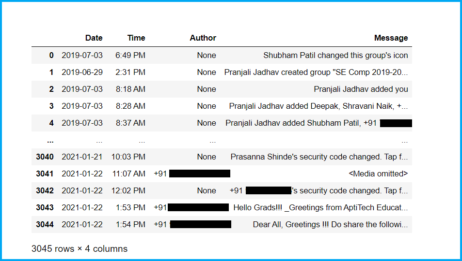
Now, let's check the basic information of our dataset and clean the dataset:
### Checking shape of dataseta "dataset" or dataset is a structured collection of information, which can be used for statistical analysis, Machine learning or research. Datasets can include numerical variables, categorical or textual, and their quality is crucial for reliable results. Its use extends to various disciplines, such as medicine, economics and social science, facilitating informed decision-making and the development of predictive models.....
df.shape
### Checking basic information of dataset
df.info()
### Checking no. of nullThe term "NULL" It is used in programming and databases to represent a null or non-existent value. Its main function is to indicate that a variable does not have a value assigned to it or that a piece of data is not available. And SQL, for instance, Used to manage records that lack information in certain columns. Understanding the use of "NULL" It is essential to avoid errors in data manipulation and... values in dataset
df.isnull().sum()
### Checking head part of dataset
df.head(50)
### Checking tail part of dataset
df.tail(50)
### Droping Nan values from dataset
df = df.dropna()
df = df.reset_index(drop=True)
df.shape
### Checking no. of authors of group
df['Author'].nuniquam()
### Checking authors of group
df['Author'].unique()
Now, we pre-process our data set and try to extract useful information from it:
### Adding one more column of "Day" for better analysis, here we use datetime library which help us to do this task easily.
weeks = {
0 : 'Monday',
1 : 'Tuesday',
2 : 'Wednesday',
3 : 'Thrusday',
4 : 'Friday',
5 : 'Saturday',
6 : 'Sunday'
}
df['Day'] = df['Date'].dt.weekday.map(weeks)
### Rearranging the columns for better understanding
df = df[['Date','Day','Time','Author','Message']]
### Changing the datatype of column "Day".
df['Day'] = df['Day'].astype('category')
### Looking newborn dataset.
df.head()
### Counting number of letters in each message
df['Letter's'] = df['Message'].apply(lambda s : len(s))
### Counting number of word's in each message
df['Word's'] = df['Message'].apply(lambda s : len(s.split(' ')))
### Function to count number of links in dataset, it will add extra column and store information in it.
URLPATTERN = r'(https?://S+)'
df['Url_Count'] = df.Message.apply(lambda x: re.findall(URLPATTERN, x)).str.len()
links = np.sum(df.Url_Count)
### Function to count number of media in chat.
MEDIAPATTERN = r'<Media omitted>'
df['Media_Count'] = df.Message.apply(lambda x : re.findall(MEDIA PATTERN, x)).str.len()
media = np.sum(df.Media_Count)
### Looking updated dataset
df
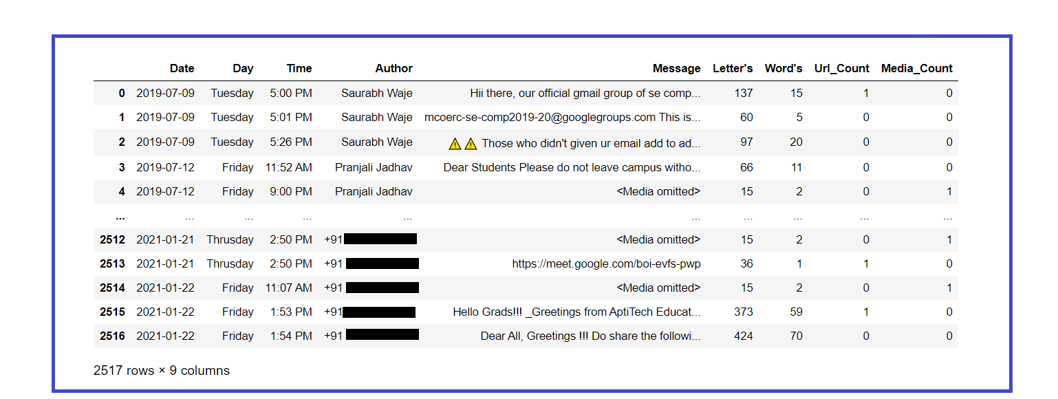
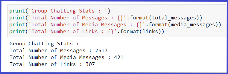
Extract basic statistics from the dataset:
total_messages = df.shape[0]
media_messages = df[df['Message'] == '<Media omitted>'].shape[0]
links = np.sum(df.Url_Count)
print('Group Chatting Stats : ')
print('Total Number of Messages : {}.format(total_messages))
print('Total Number of Media Messages : {}.format(media_messages))
print('Total Number of Links : {}.format(links))
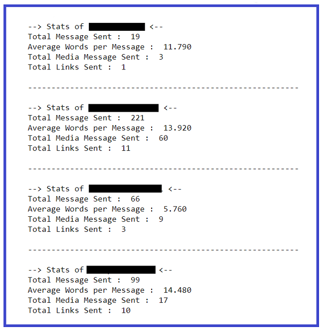
Extracting basic statistics from each user:
l = df.Author.unique()
for i in range(len(l)):
  ### Filtering out messages of particular user
  req_df = df[df["Author"] == l[i]]
  ### req_df will contain messages of only one particular user
  print(f'--> Stats of {l[i]} <-- ')
  ### shape will print number of rows which indirectly means the number of messages
  print('Total Message Sent : ', req_df.shape[0])
  ### Word_Count contains of total words in one message. Sum of all words/ Total Messages will yield words per message
  words_per_message = (np.sum(req_df['Word's']))/req_df.shape[0]
  w_p_m = ("%.3f" % round(words_per_message, 2))
  print('Average Words per Message : ', w_p_m)
  ### media conists of media messages
  media = sum(req_df["Media_Count"])
  print('Total Media Message Sent : ', media)
  ### links consist of total links
  links = sum(req_df["Url_Count"])
  print('Total Links Sent : ', links)
  print()
  print('----------------------------------------------------------n')
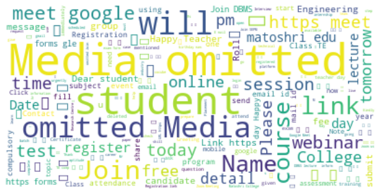
Let's create a word cloud with the most used words in the chat:
### Word Cloud of mostly used word in our Group
text = " ".join(review for review in df.Message)
wordcloud = WordCloud(stopwords=STOPWORDS, background_color="white").generate(text)
  ### Display the generated image:
plt.figure( figsize=(10,5))
plt.imshow(wordcloud, interpolation='bilinear')
plt.axis("off")
plt.show()
Let's print the total no.. of messages sent by each user:
### Creates a list of unique Authors
l = df.Author.unique()
for i in range(len(l)):
  ### Filtering out messages of particular user
  req_df = df[df["Author"] == l[i]]
  ### req_df will contain messages of only one particular user
  print(l[i],'  ->  ',req_df.shape[0])
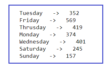
We print the total of messages sent each day of the week:
l = df.Day.unique()
for i in range(len(l)):
  ### Filtering out messages of particular user
  req_df = df[df["Day"] == l[i]]
  ### req_df will contain messages of only one particular user
  print(l[i],'  ->  ',req_df.shape[0])
Finally, we have extracted enough text information from the chat file, Now let's start the Data Visualization part that will help us for a better analysis and understanding of all the analysis we have done on our exported chat file. In the place of contact numbers, I have used alphabets for security reasons, very sorry.
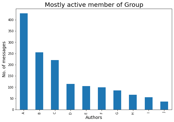
Let's see who is the most active author of the group:
### Mostly Active Author in the Group
plt.figure(figsize=(9,6))
mostly_active = df['Author'].value_counts()
### Top 10 peoples that are mostly active in our Group is :
m_a = mostly_active.head(10)
bars = ['A','B','C','D','E','F','G','H','I','J']
x_pos = np.arange(len(bars))
m_a.plot.bar()
plt.xlabel('Authors',fontdict={'fontsize': 14,'fontweight': 10})
plt.ylabel('No. of messages',fontdict={'fontsize': 14,'fontweight': 10})
plt.title('Mostly active member of Group',fontdict={'fontsize': 20,'fontweight': 8})
plt.xticks(x_pos, bars)
plt.show()
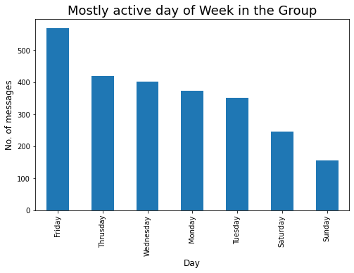
Let's look at the most active day in a week:
### Mostly Active day in the Group
plt.figure(figsize=(8,5))
active_day = df['Day'].value_counts()
### Top 10 peoples that are mostly active in our Group is :
a_d = active_day.head(10)
a_d.plot.bar()
plt.xlabel('Day',fontdict={'fontsize': 12,'fontweight': 10})
plt.ylabel('No. of messages',fontdict={'fontsize': 12,'fontweight': 10})
plt.title('Mostly active day of Week in the Group',fontdict={'fontsize': 18,'fontweight': 8})
plt.show()
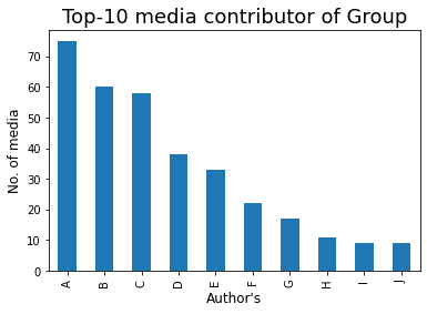
Let's look at the Top-10 media contributor in the group:
### Top-10 Media Contributor of Group
mm = df[df['Message'] == '<Media omitted>']
mm1 = mm['Author'].value_counts()
bars = ['A','B','C','D','E','F','G','H','I','J']
x_pos = np.arange(len(bars))
top10 = mm1.head(10)
top10.plot.bar()
plt.xlabel('Author's',fontdict={'fontsize': 12,'fontweight': 10})
plt.ylabel('No. of media',fontdict={'fontsize': 12,'fontweight': 10})
plt.title('Top-10 media contributor of Group',fontdict={'fontsize': 18,'fontweight': 8})
plt.xticks(x_pos, bars)
plt.show()
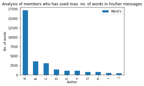
The words are, of course, the most powerful weapon in the world, so let's see who has this mighty weapon in the group😅:
max_words = df[['Author','Word's']].groupby('Author').sum()
m_w = max_words.sort_values('Word's',ascending=False).head(10)
bars = ['A','B','C','D','E','F','G','H','I','J']
x_pos = np.arange(len(bars))
m_w.plot.bar(rot=90)
plt.xlabel('Author')
plt.ylabel('No. of words')
plt.title('Analysis of members who has used max. no. of words in his/her messages')
plt.xticks(x_pos, bars)
plt.show()
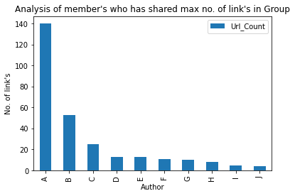
Let's look at the Top-10 author who has shared the maximum number. of links in the group:
### Member who has shared max numbers of link in Group
max_words = df[['Author','Url_Count']].groupby('Author').sum()
m_w = max_words.sort_values('Url_Count',ascending=False).head(10)
bars = ['A','B','C','D','E','F','G','H','I','J']
x_pos = np.arange(len(bars))
m_w.plot.bar(rot=90)
plt.xlabel('Author')
plt.ylabel('No. of link's')
plt.title('Analysis of member's who has shared max no. of link's in Group')
plt.xticks(x_pos, bars)
plt.show()
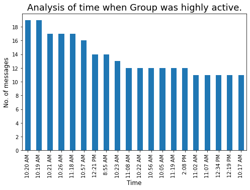
Let's see the time each time the group was very active:
### Time whenever our group is highly active
plt.figure(figsize=(8,5))
t = df['Time'].value_counts().head(20)
tx = t.plot.bar()
tx.yaxis.set_major_locator(MaxNLocator(integer=True))  #Converting y axis data to integer
plt.xlabel('Time',fontdict={'fontsize': 12,'fontweight': 10})
plt.ylabel('No. of messages',fontdict={'fontsize': 12,'fontweight': 10})
plt.title('Analysis of time when Group was highly active.',fontdict={'fontsize': 18,'fontweight': 8})
plt.show()
Format conversion 12 hours to 24 hours will help us perform a better analysis:
lst = []
for i in df['Time'] :
out_time = datetime.strftime(datetime.strptime(i,"%I:%M %p"),"%H:%M")
lst.append(out_time)
df['24H_Time'] = lst
df['Hours'] = df['24H_Time'].apply(lambda x : x.split(':')[0])
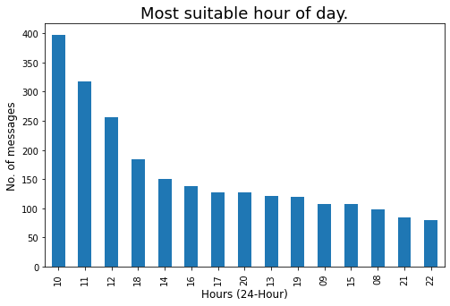
Let's review the most appropriate time of day when there is a better chance of getting a response from group members:
### Most suitable hour of day, whenever there will more chances of getting responce from group members.
plt.figure(figsize=(8,5))
std_time = df['Hours'].value_counts().head(15)
s_T = std_time.plot.bar()
s_T.yaxis.set_major_locator(MaxNLocator(integer=True))  #Converting y axis data to integer
plt.xlabel('Hours (24-Hour)',fontdict={'fontsize': 12,'fontweight': 10})
plt.ylabel('No. of messages',fontdict={'fontsize': 12,'fontweight': 10})
plt.title('Most suitable hour of day.',fontdict={'fontsize': 18,'fontweight': 8})
plt.show()
Let's create a word cloud of the 10 most active members:
active_m = [list of Top-10 highly active members]
for i in range(len(active_m)) :
    # Filtering out messages of particular user
    m_chat = df[df["Author"] == active_m[i]]
    print(f'--- Author :  {active_m[i]} --- ')
    # Word Cloud of mostly used word in our Group
    msg = ' '.join(x for x in m_chat.Message)
    wordcloud = WordCloud(stopwords=STOPWORDS, background_color="white").generate(msg)
    plt.figure(figsize=(10,5))
    plt.imshow(wordcloud, interpolation='bilinear')
    plt.axis("off")
    plt.show()
    print('____________________________________________________________________________________n')
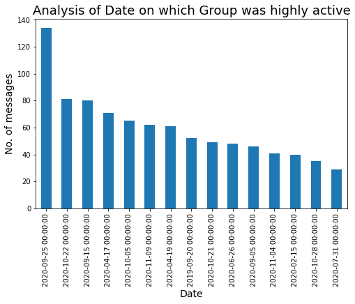
Let's see the date our group was very active:
### Date on which our Group was highly active.
plt.figure(figsize=(8,5))
df['Date'].value_counts().head(15).plot.bar()
plt.xlabel('Date',fontdict={'fontsize': 14,'fontweight': 10})
plt.ylabel('No. of messages',fontdict={'fontsize': 14,'fontweight': 10})
plt.title('Analysis of Date on which Group was highly active',fontdict={'fontsize': 18,'fontweight': 8})
plt.show()
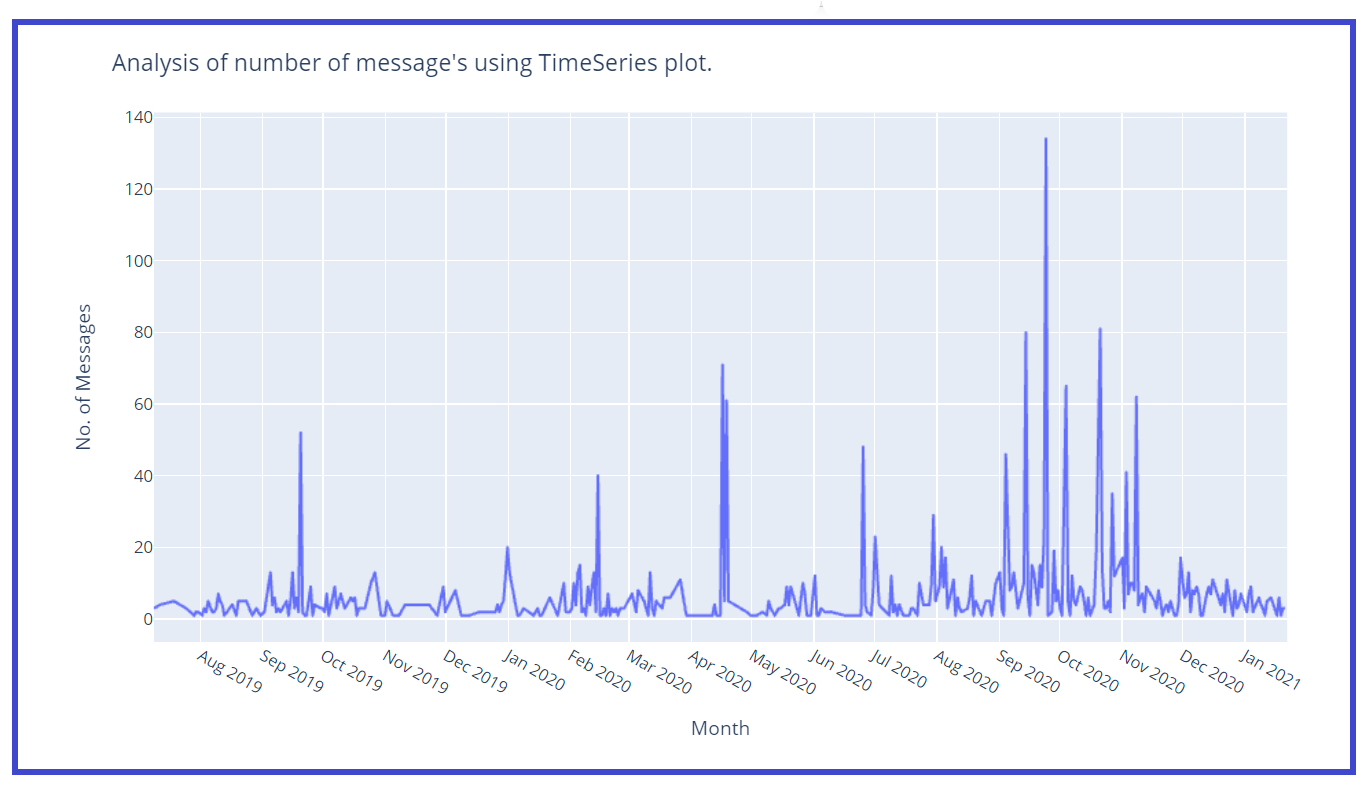
Let's create a time series graph wrt no. of messages:
z = df['Date'].value_counts()
z1 = z.to_dict() #converts to dictionary
df['Msg_count'] = df['Date'].map(z1)
### Timeseries plot
fig = px.line(x=df['Date'],y = df['Msg_count'])
fig.update_layout(title="Analysis of number of message"s using TimeSeries plot.',
                  xaxis_title="Month",
                  yaxis_title="No. of Messages")
fig.update_xaxes(nticks=20)
fig.show()
Let's create a separate column for Month and Year for better analysis:
df['Year'] = df['Date'].dt.year
df['Mon'] = df['Date'].dt.month
months = {
     1 : 'Jan',
     2 : 'Feb',
     3 : 'Mar',
     4 : 'Apr',
     5 : 'May',
     6 : 'Jun',
     7 : 'Jul',
     8 : 'Aug',
     9 : 'Sep',
    10 : 'Oct',
    11 : 'Nov',
    12 : 'Dec'
}
df['Month'] = df['Mon'].map(months)
df.drop('Mon',axis=1,inplace=True)
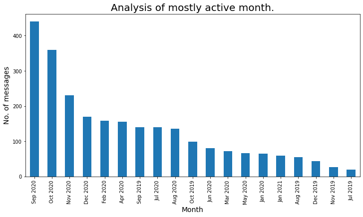
Let's look at the most active month:
### Mostly Active month
plt.figure(figsize=(12,6))
active_month = df['Month_Year'].value_counts()
a_m = active_month
a_m.plot.bar()
plt.xlabel('Month',fontdict={'fontsize': 14,'fontweight': 10})
plt.ylabel('No. of messages',fontdict={'fontsize': 14,'fontweight': 10})
plt.title('Analysis of mostly active month.',fontdict={'fontsize': 20,
        'fontweight': 8})
plt.show()
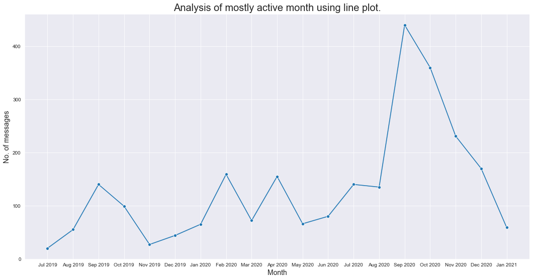
Let's analyze the busiest month using a line diagram:
z = df['Month_Year'].value_counts()
z1 = z.to_dict() #converts to dictionary
df['Msg_count_monthly'] = df['Month_Year'].map(z1)
plt.figure(figsize=(18,9))
sns.set_style("darkgrid")
sns.lineplot(data=df,x='Month_Year',y='Msg_count_monthly',markers=True,marker="O")
plt.xlabel('Month',fontdict={'fontsize': 14,'fontweight': 10})
plt.ylabel('No. of messages',fontdict={'fontsize': 14,'fontweight': 10})
plt.title('Analysis of mostly active month using line plot.',fontdict={'fontsize': 20,'fontweight': 8})
plt.show()
Let's review the total message per year:
### Total message per year
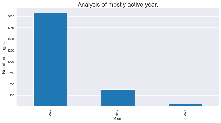
### As we analyse that the group was created in mid 2019, thats why number of messages in 2019 is less.
plt.figure(figsize=(12,6))
active_month = df['Year'].value_counts()
a_m = active_month
a_m.plot.bar()
plt.xlabel('Year',fontdict={'fontsize': 14,'fontweight': 10})
plt.ylabel('No. of messages',fontdict={'fontsize': 14,'fontweight': 10})
plt.title('Analysis of mostly active year.',fontdict={'fontsize': 20,'fontweight': 8})
plt.show()
Let's use a heat mapa "heat map" is a graphical representation that uses colors to show the density of data in a specific area. Commonly used in data analytics, Marketing and behavioral studies, This type of visualization allows you to identify patterns and trends quickly. Through chromatic variations, Heat maps make it easier to interpret large volumes of information, helping to make informed decisions.... and let's analyze the time of day with great activity:
df2 = df.groupby(['Hours', 'Day'], as_index=False)["Message"].count()
df2 = df2.dropna()
df2.reset_index(drop = True,inplace = True)
### Analysing on which time group is mostly active based on hours and day.
analysis_2_df = df.groupby(['Hours', 'Day'], as_index=False)["Message"].count()
### Droping null values
analysis_2_df.dropna(inplace=True)
analysis_2_df.sort_values(by=['Message'],ascending=False)
day_of_week = ['Monday', 'Tuesday', 'Wednesday', 'Thrusday', 'Friday', 'Saturday', 'Sunday']
plt.figure(figsize=(15,8))
heatmap(
    x=analysis_2_df['Hours'],
    y=analysis_2_df['Day'],
    size_scale = 500,
    size = analysis_2_df['Message'],
    y_order = day_of_week[::-1],
    color = analysis_2_df['Message'],
    palette = sns.cubehelix_palette(128)
)
plt.show()
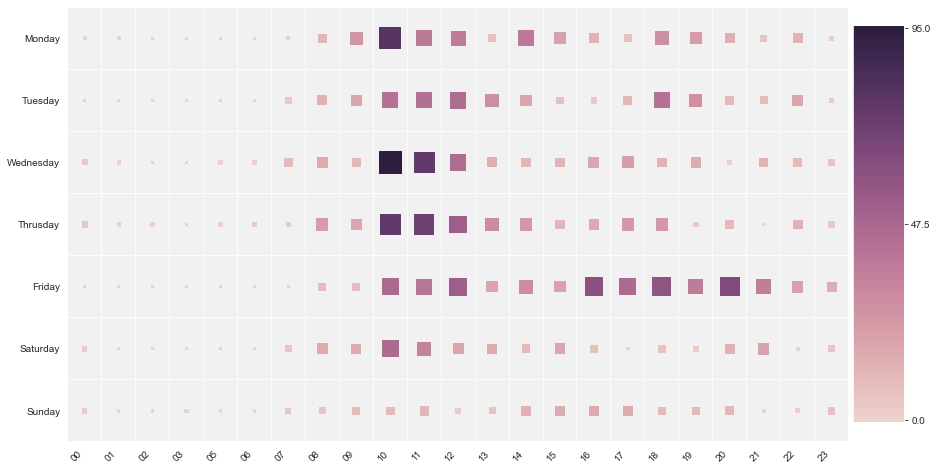
From the heat map above, we analyze that the “Monday” between the 10:00 and the 10:59, our group was
very active, similarly the “Wednesday” between the 10:00 and the 10:59, our group was
highly active. Between the 00:00 and the 08:00 the group was less active.
Final note:
Hope this article really helps you create your own WhatsApp chat analyzer and analyze the pattern in the group.
Hope you enjoyed this article. Any question? Have i missed something? Please contact me at my LinkedIn. And finally, … No need to say,
Thank you for reading!
Health!!!
Ronil
The media shown in this article is not the property of DataPeaker and is used at the author's discretion.





