Time series prediction methods | Arima in Python and R

Introduction

Imagine this: you have been tasked with forecasting the price of the next iPhone and provided with historical data. This includes features like quarterly sales, monthly expenses and a host of things that come with Apple's balance sheet. As a data scientist, What kind of problem would you classify this into? Time series modeling, of course.

From predicting product sales to estimating household electricity use, time series prediction is one of the core skills any data scientist is expected to know, if not that dominate. There are a plethora of different techniques you can use, and in this article we will cover one of the most effective, called Auto ARIMA.

We will first understand the concept of ARIMA which will lead us to our main topic: Auto ARIMA. To solidify our concepts, we will take a dataset and implement it in both Python and R.

Table of Contents

1. What is a time series?
2. Methods for forecasting time series
3. Introduction to ARIMA
4. Steps to implement ARIMA
5. Why do we need AutoARIMA?
6. ARIMA Automatic Implementation (in the air passenger dataset)
7. How do you select auto ARIMA parameters?

If you are familiar with time series and their techniques (as moving average, exponential smoothing and ARIMA), you can go directly to the section 4. For starters, start from the section below, which is a brief introduction to time series and various forecasting techniques. .

1. What is a time series?

Before learning about techniques for working with time series data, we must first understand what a time series really is and how it differs from any other data type. Here is the formal definition of time series: is a series of data points measured in consistent time intervals. This simply means that particular values ​​are recorded at a constant interval which can be hourly., daily, weekly, every 10 days, etc. What makes time series different is that each data point in the series depends on the previous data points. Let's understand the difference more clearly by taking a couple of examples.

Example 1:

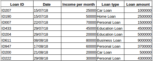
Suppose you have a data set of people who have obtained a loan from a particular company (as shown in the following table). Do you think that each row will be related to the previous rows? Certainly not! The loan taken by a person will be based on their financial conditions and needs (there could be other factors such as family size, etc., but to simplify we are considering only the income and the type of loan). What's more, data was not collected in any specific time interval. It depends on when the company received a loan application.

Example 2:

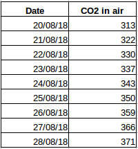
Let's take another example. Suppose you have a data set that contains the level of CO2 in the air per day (screenshot below). Can you predict the approximate amount of CO2 for the next day by looking at the values ​​for the last few days? Good, of course. If you notice, data has been recorded daily, namely, the time interval is constant (24 hours).

You must have had an intuition on this by now: the first case is a simple regression problem and the second is a time series problem. Although the time series puzzle here can also be solved using linear regression, that's not really the best approach, since it neglects the relation of the values ​​with all the relative past values. Let's now look at some of the common techniques used to solve time series problems..

2. Methods for forecasting time series

There are several methods for time series forecasting and we will cover them briefly in this section.. Detailed explanation and Python codes for all techniques mentioned below can be found in this article: 7 techniques for forecasting time series (with python codes).

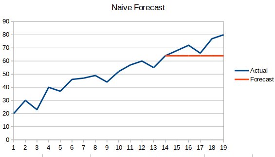
1. Naive approach: In this forecasting technique, the value of the new data point is predicted to be equal to the previous data point. The result would be a flat line, since all the new values ​​take the previous values.
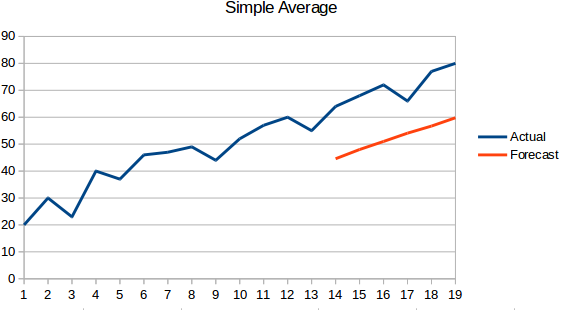
2. Simple average: The following value is taken as the average of all previous values. The predictions here are better than the 'Naive Approach', as it does not result in a flat line, but here, all past values ​​are taken into consideration, what may not always be useful. For instance, when asked to predict today's temperature, I would consider the temperature of the last 7 days instead of the temperature of a month ago.
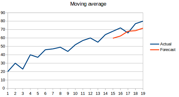
3. Moving average : This is an improvement over the prior art. Instead of taking the average of all the above points, the average of 'n’ above points is taken as the predicted value.
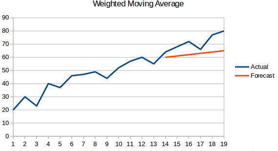
4. Weighted moving average: A weighted moving average is a moving average in which the values' n’ past are given different weights.
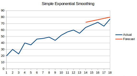
5. Simple exponential smoothing: In this technique, more recent observations are assigned greater weights than those of the distant past.
6. Holt's linear trend model: This method takes into account the trend of the data set. By trend, we mean the increasing or decreasing nature of the series. Suppose the number of hotel reservations increases every year, then we can say that the number of reservations shows an increasing trend. The forecast function in this method is a level and trend function.
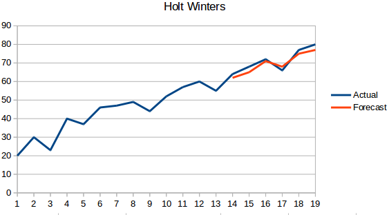
7. Holt Winters method: This algorithm takes into account both the trend and the seasonality of the series. For instance, the number of hotel reservations is high on weekends and low on weekdays, and increases every year; there is a weekly seasonality and a growing trend.
8. ARIMA: ARIMA is a very popular technique for time series modeling. Describes the correlation between data points and takes into account the difference in values. An improvement over ARIMA is SARIMA (o Seasonal ARIMA). We will look at ARIMA in a little more detail in the next section..

3. Introduction to ARIMA

In this section we will make a quick introduction to ARIMA that will be useful to understand Auto Arima. A detailed explanation of Arima is included in this article, parameters (p, q, d), graphics (ACF PACF) and implementation: Complete time series tutorial.

ARIMA is a very popular statistical method for forecasting time series. ARIMA means Integrated auto-regressive moving averages. ARIMA models work with the following assumptions:

• The data series is stationary, which means that the mean and variance must not vary over time. A series can be made stationary using logarithmic transformation or by differentiating the series.
• The data provided as input must be a univariate series, since arima uses past values ​​to predict future values.

ARIMA has three components: WITH (autoregressive term), I (differentiation term) y MA (moving average term). Let's understand each of these components:

• The term AR refers to the past values ​​used to forecast the next value. The term AR is defined by the parameter 'p’ in arima. The value of 'p’ determined using the PACF chart.
• The term MA is used to define the number of past forecast errors that are used to predict future values. The 'q parameter’ in arima it represents the term MA. The ACF chart is used to identify the value 'q’ Right.
• The differentiation order specifies the number of times the serial differentiation operation is performed to make it stationary. Tests such as ADF and KPSS can be used to determine if the series is stationary and help identify the d-value.

4. Steps to implement ARIMA

The general steps to implement an ARIMA model are:

1. Upload the data: The first step in model building is, of course, load dataset.
2. Preprocessing: Depending on the data set, the preprocessing steps will be defined. This will include creating timestamps, convert date column type / time, make the series univariate, etc.
3. Make the series stationary: To satisfy the assumption, it is necessary to make the series stationary. This would include checking the stationarity of the series and performing the necessary transformations.
4. Determine the value d: To make the series stationary, the number of times the difference operation was performed will be taken as the value d
5. Create ACF and PACF charts: This is the most important step in the implementation of ARIMA. The ACF PACF charts are used to determine the input parameters for our ARIMA model.
6. Determine the p and q values: Read the p and q values ​​from the graphs of the previous step
7. Fit the ARIMA model: Using the processed data and the parameter values ​​that we calculated from the previous steps, fit the ARIMA model
8. Predict values ​​in the validation set: Predicting future values
9. Calculate RMSE: To verify the performance of the model, check RMSE value using predictions and actual values ​​in validation set.

5. Why do we need Auto ARIMA?

Although ARIMA is a very powerful model for forecasting time series data, data preparation and parameter tuning processes end up consuming a lot of time. Before implementing ARIMA, you need to make the series stationary and determine the values ​​of p and q using the graphs we discussed earlier. Auto ARIMA makes this task really easy for us, since it eliminates the steps 3 a 6 that we saw in the previous section. Then, the steps you need to follow to implement automatic ARIMA are shown:

1. Load data: This step will be the same. Upload the data to your laptop
2. Data pre-processing: input must be univariate, Thus, remove the other columns
3. Fit Auto ARIMA: fits the model on the univariate series
4. Predict values ​​in the validation set: make predictions on the validation set
5. Calculate RMSE: check model performance using predicted values ​​against actual values

We completely ignore the selection of functions p and q, as you can see. What a relief! In the next section, we will implement auto ARIMA using a toy dataset.

6. Implementation in Python and R

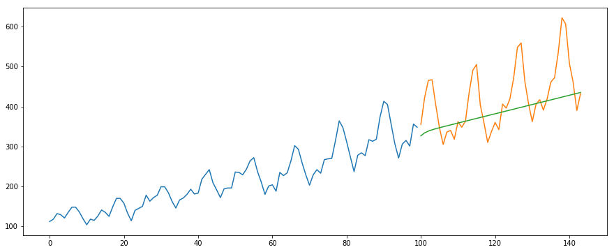
We will use the International-Air-Passenger dataset. This data set contains the total monthly number of passengers (in thousands). It has two columns: month and passenger count. You can download the dataset from this link.

#load the data
data = pd.read_csv('international-airline-passengers.csv')

#divide into train and validation set
train = data[:int(0.7*(len(data)))]
valid = data[int(0.7*(len(data))):]

#preprocessing (since arima takes univariate series as input)
train.drop('Month',axis=1,inplace=True)
valid.drop('Month',axis=1,inplace=True)

#plotting the data
train['International airline passengers'].plot()
valid['International airline passengers'].plot()

#building the model
from pyramid.arima import auto_arima
model = auto_arima(train, trace=True, error_action='ignore', suppress_warnings=True)
model.fit(train)

forecast = model.predict(n_periods = only(valid))
forecast = pd.DataFrame(forecast,index = valid.index,columns=['Prediction'])

#plot the predictions for validation set
plt.plot(train, label="Train")
plt.plot(valid, label="Valid")
plt.plot(forecast, label="Prediction")
plt.show()

#calculate rmse
from math import sqrt
from sklearn.metrics import mean_squared_error

rms = sqrt(mean_squared_error(valid,forecast))
print(rms)

output -
76.51355764316357

Below is the R code for the same problem:

# loading packages
library(forecast)
library(Metrics)

# reading data
data = read.csv("international-airline-passengers.csv")

# splitting data into train and valid sets
train = data[1:100,]
valid = data[101:nrow(data),]

# removing "Month" column
train$Month = NULL

# training model
model = auto.arima(train)

# model summary
summary(model)

# forecasting
forecast = predict(model,44)

# evaluation
rmse(valid$International.airline.passengers, forecast$pred)

7. How does Auto Arima select the best parameters?

In the above code, we just use the .to fit in() command to fit the model without having to select the combination of p, q, d. But, How did the model discover the best combination of these parameters? Auto ARIMA takes into account the AIC and BIC values ​​generated (as you can see in the code) to determine the best combination of parameters. AIC values (Akaike Information Criterion) y BIC (Bayesian Information Criterion) are estimators to compare models. The lower these values ​​are, the better the model.

Check out these links if you are interested in the math behind AIC Y BIC.

8. Final notes and further reading

I have found auto ARIMA to be the simplest technique for making time series forecasting. Knowing a shortcut is good, but it is also important to be familiar with the math behind it. In this article, I have examined the details of how ARIMA works, but be sure to check out the links provided in the article. For your easy reference, here are the links again:

I would suggest practicing what we have learned here about this practice problem: Time series practice problem. You can also take our training course created on the same practice problem, Forecasting time series, to give you a head start.

Good luck and feel free to send us your comments and ask questions in the comment section below..

Related