
Introduction
Data manipulation is an inevitable phase of predictive modeling. A robust predictive model cannot be built simply using machine learning algorithms. But, with an approach to understanding the business problem, the underlying data, perform the necessary data manipulations and then extract business information.
Among these various phases of model building, most of the time is usually spent understanding the underlying data and performing the necessary manipulations. This would also be the central theme of this article: packages for faster data manipulation in R.
What is data manipulation?
If you are still confused with this 'term', let me explain. Data manipulation is a term that is used loosely with “Data exploration”. It implies to manipulate’ data using a set of available variables. This is done to improve the accuracy and precision associated with the data..
In reality, the data collection process can have many gaps. There are several uncontrollable factors that lead to inaccuracy in the data, as the mental situation of the respondents, personal biases, differences / errors in machine readings, etc. To mitigate these inaccuracies, data is manipulated to increase accuracy (maximum) possible in the data.
Sometimes, this stage is also known as data dispute or data cleansing.
Different ways to manipulate / process data:
There is no right or wrong way to manipulate data, as long as you understand them and have taken the necessary actions at the end of the exercise. But nevertheless, here are some general ways that people try to approach data manipulation. Are here:
- As usual, beginners in R are comfortable manipulate data using built-in base R functions. This is a good first step., but it is often repetitive and time consuming. Therefore, is a less efficient way to solve the problem.
- Using packages for data manipulation. CRAN has more than 7000 packages currently available. In simple words, these packages are nothing more than a collection of commonly used pre-written codes. Help you perform repetitive tasks on an empty stomach, reduce coding errors and get help from expertly written code (across the open source ecosystem for R) to make your code more efficient. This is usually the most common way to perform data manipulation.
- Use of ML algorithms for data manipulation. You can use tree-based reinforcement algorithms to deal with missing data and outliers. While these definitely require less time, these approaches usually leave you wanting a better understanding of the data in the end.
Therefore, Most of the time, the use of packages is the de facto method to perform data manipulation. In this article, I have explained several packages that make ‘R’s life easier’ during the data manipulation stage.
Note: This article is more suitable for beginners in R Language. You can install a package using:
install.packages('package name')
Package list
For a better understanding, I have also demonstrated its use by performing commonly used operations. Below is the list of packages discussed in this article:
- dplyr
- data table
- ggplot2
- remodelar2
- reader
- tidyr
- lubridate
Note: I understand that ggplot2 is a graphical package. But, in general, helps to visualize data (distributions, correlations) and perform manipulations accordingly. Therefore, i added it to this list. In all packages, I have covered only the most used commands in data manipulation.
dplyr package
These packages are created and maintained by Hadley Wickham. This package has everything (almost) to speed up your data manipulation efforts. He is best known for data exploration and transformation. Its chaining syntax makes it highly customizable to use. It includes 5 main data manipulation commands:
- filter: filter data based on a condition
- to select: used to select columns of interest from a data set
- Organize: is used to organize the dataset values in ascending or descending order.
- twirl: used to create new variables from existing variables
- abstract (con group_by): used to perform analysis using commonly used operations, As minimum, maximum, mean count, etc.
Focus on these commands and do a great job exploring data. Let's understand these commands one by one. I have used 2 pre-installed R datasets, namely, mtcars e iris.
> library(dplyr)
> data("mtcars")
> data('iris')
> mydata <- mtcars
#read data
> head(mydata)

#creating a local dataframe. Local data frame are easier to read

> access data <- tbl_df(mydata)
> myirisdata <- tbl_df(iris)
#now data will be in tabular structure > access data> myirisdata
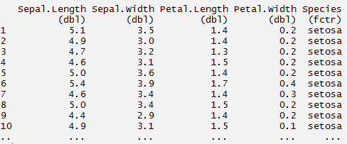
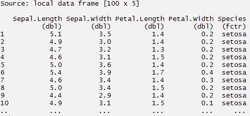
#use filter to filter data with required condition > filter(access data, cyl > 4 & gear > 4 )> filter(access data, cyl > 4)
> filter (myirisdata, Species% in% c ('setosa', 'virginica'))
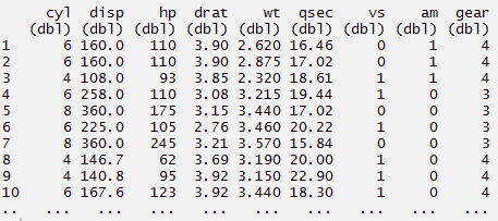
#use selectThe command "SELECT" is fundamental in SQL, used to query and retrieve data from a database. Allows you to specify columns and tables, filtering results using clauses such as "WHERE" and ordering with "ORDER BY". Its versatility makes it an essential tool for data manipulation and analysis, facilitating the obtaining of specific information efficiently.... to pick columns by name > select(access data, cyl,mpg,hp)#here you can use (-) to hide columns > select(access data, -cyl, -mpg )
# hide a range of columns> to select (access data, -c (cyl, mpg))
#chaining or pipelining - a way to perform multiple operations
#in one line
> access%>%
     select(cyl, wt, gear)%>%
     filter(wt > 2)
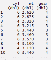
#arrange can be used to reorder rows
> access%>%
     select(cyl, wt, gear)%>%
     arrange(wt)
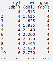
#or
> access%>%
     select(cyl, wt, gear)%>%
     arrange(desc(wt))
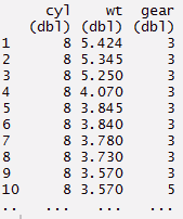
#mutate - create new variables

> access%>%
      select(mpg, cyl)%>%
      mutate(newvariable = mpg*cyl)
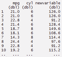
#or
> newvariable <- access%>% mutate(newvariable = mpg*cyl)
#summarise - this is used to find insights from data
> myirisdata%>%
       group_by(Species)%>%
       summarise(Average = mean(Sepal.Length, na.rm = TRUE))
#or use summarise each
> myirisdata%>%
group_by(Species)%>%
summarise_each(funs(mean, n()), Sepal.Length, Sepal.Width)
 #You can create complex chain commands using these 5 verbs.
#you can rename the variables using rename command
> access%>% rename(miles = mpg)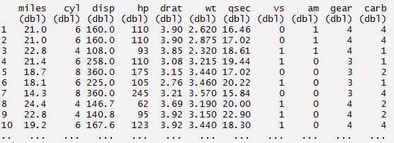
data.table package
This package allows you to perform faster manipulation on a data set. Ditch your traditional ways of sub-configuring rows and columns and use this package. With minimal coding, can do much more. Using data.table helps reduce computation time compared to data.frame. You will be amazed by the simplicity of this package.
A data table has 3 parts, namely, DT[i,j,by]. You can understand this as, we can tell R to make a subset of the rows using 'i', to calculate ‘j’ which is grouped by 'by'. Most of the time, “by” se relaciona con una variableIn statistics and mathematics, a "variable" is a symbol that represents a value that can change or vary. There are different types of variables, and qualitative, that describe non-numerical characteristics, and quantitative, representing numerical quantities. Variables are fundamental in experiments and studies, since they allow the analysis of relationships and patterns between different elements, facilitating the understanding of complex phenomena.... Categorical. In the following code, I have used 2 data sets (air quality and iris).
#load data
> data("airquality")
> mydata <- airquality
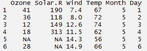
> head(airquality,6)
> data(iris)
> myiris <- iris
#load package
> library(data.table)
> mydata <- data.table(mydata)
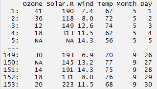
> mydata
> myiris <- data.table(myiris)
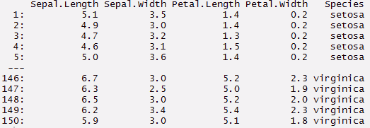
> myiris
#subset rows - select 2nd to 4th row

> mydata[2:4,]
#select columns with particular values
> myiris[Species == 'setosa']
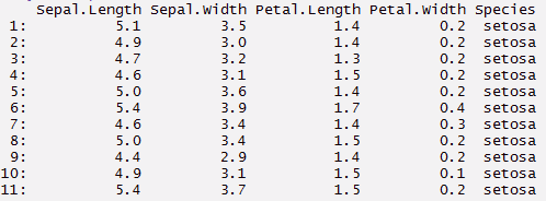
#select columns with multiple values. This will give you columns with Setosa
#and virginica species
> myiris[Species %in% c('setosa', 'virginica')]

#select columns. Returns a vector
> mydata[,Temp]
> mydata[,.(Temp,Month)]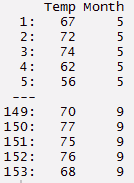
#returns sum of selected column
> mydata[,sum(Ozone, na.rm = TRUE)]

[1]4887
#returns sum and standard deviation
> mydata[,.(sum(Ozone, na.rm = TRUE), sd(Ozone, na.rm = TRUE))]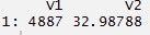
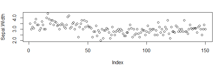
#print and plot
> myiris[,{print(Sepal.Length)
> plot(Sepal.Width)
 NULL}]

#grouping by a variable
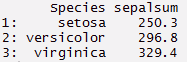
> myiris[,.(sepalsum = sum(Sepal.Length)), by=Species]
#select a column for computation, hence need to set the key on column
> setkey(myiris, Species)

#selects all the rows associated with this data point
> myiris['setosa']
> myiris[c('setosa', 'virginica')]
Ggplot2 package
ggplot offers a whole new world of colors and patterns. If you are a creative soul, you will love this pack to the core. But, if you want to learn what is necessary to get started, follow the codes below. You must learn the ways to trace at least these 3 graphics: Dispersion diagramThe scatter plot is a graphical tool used in statistics to visualize the relationship between two variables. It consists of a set of points in a Cartesian plane, where each point represents a pair of values corresponding to the variables analyzed. This type of chart allows you to identify patterns, Trends and possible correlations, facilitating data interpretation and decision-making based on the visual information presented...., Bar chart, Histogram.
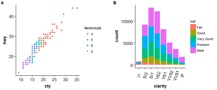
These 3 chart patterns cover almost all types of data representation, except maps. ggplot is enriched with custom functions to make your viewing better and better. It becomes even more powerful when bundled with other packages like cowplot, gridExtra. In fact, there are many functions. Therefore, you need to focus on a few commands and develop your expertise in them. I have also shown the method to compare charts in a window. Requires the 'gridExtra' package. Therefore, must install it. I used pre-installed R datasets.
> library(ggplot2)
> library(gridExtra)
> df <- ToothGrowth
> df$dose <- as.factor(df$dose)
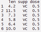
> head(df)
#boxplot
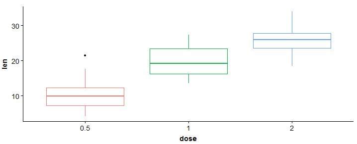
> bp <- ggplot(df, aes(x = dose, y = len, color = dose)) + geom_boxplot() + theme(legend.position = 'none')
> bp
#add gridlines
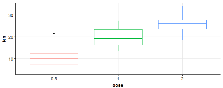
> bp + background_grid(major = "xy", minor="none")
#scatterplot
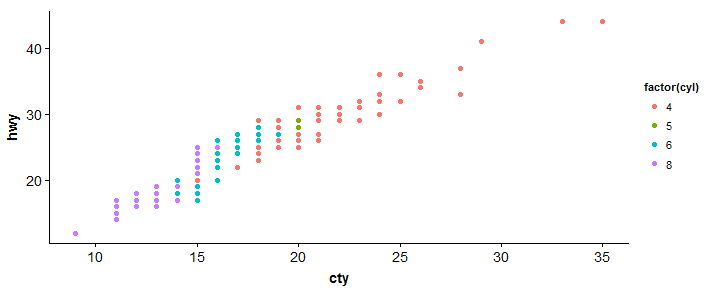
> sp <- ggplot(mpg, aes(x = ct, y = hwy, color = factor(cyl)))+geom_point(size = 2.5)
> sp
#bar plot
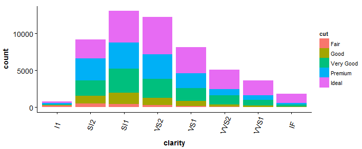
> bp <- ggplot(diamonds, aes(clarity, fill = cut)) + geom_bar() +theme(axis.text.x = element_text(angle = 70, vjust = 0.5))
> bp
#compare two plots
> plot_grid(sp, bp, labels = c("A","B"), ncol = 2, nrow = 1)
 #histogram
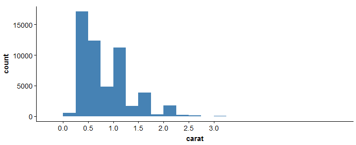
> ggplot(diamonds, aes(x = carat)) + geom_histogram(binwidth = 0.25, fill="steelblue")+scale_x_continuous(breaks=seq(0,3, by=0.5))
#histogram
> ggplot(diamonds, aes(x = carat)) + geom_histogram(binwidth = 0.25, fill="steelblue")+scale_x_continuous(breaks=seq(0,3, by=0.5))
For more information on this package, see the reference sheet here: ggplot2 cheat sheet
reshape2 package
As its name suggests, this package is useful for reshaping the data. We all know that data comes in many forms. Therefore, we are obliged to tame it according to our needs. As usual, the process of reshaping data in R is tedious and worrisome. The base functions of R consist of the option 'Aggregation’ whereby data can be reduced and reorganized into smaller forms, but with a reduction in the amount of information. Aggregation includes tapply base functions, by and added. The remodel package solves these problems. Here we try to combine features that have unique values. Has 2 functions to know melt Y to emit.
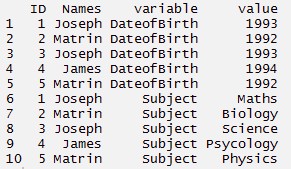
melt : This function converts data from wide format to long format. It is a form of restructuring in which multiple categorical columns are 'merged’ in unique rows. Let's understand using the code below.
#create a data
> ID <- c(1,2,3,4,5)
> Names <- c('Joseph','Matrin','Joseph','James','Matrin')
> DateofBirth <- c(1993,1992,1993,1994,1992)
> Subject<- c('Maths','Biology','Science','Psycology','Physics')
> thisdata <- data.frame(ID, Names, DateofBirth, Subject)
> data.table(thisdata)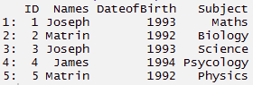
#load package
> install.packages('reshape2')
> library(reshape2)
#melt
> mt <- melt(thisdata, id=(c('ID','Names')))
> mt
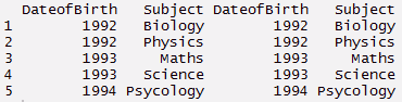
to emit : This function converts the data from long format to wide format. Starts with fused data and switches to long format. It's just the reverse of melt function. It has two functions namely, dcast Y a cast. dcast returns a data frame as output. acast returns a vector / headquarters / array as output. Let's understand using the code below.
#cast
> mcast <- dcast(mt, DateofBirth + Subject ~ variable)
> mcast
Note: While researching, I found this picture that aptly describes the remodel package.
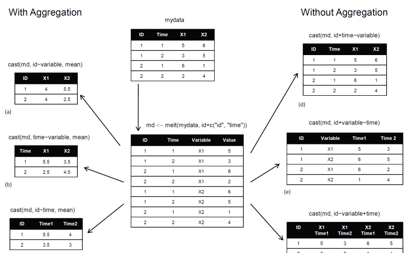 source: r-statistics
readr package
As the name suggests, ‘readr’ helps to read various forms of data in R. With a speed 10 times faster. Here, characters never become factors (so no more stringAsFactors = FALSE). This package can replace the traditional R base functions read.csv () y read.table (). Help to read the following data:
- Files delimited with
read_delim(),read_csv(),read_tsv(), Yread_csv2(). - Fixed width files with
read_fwf(), Yread_table(). - Web log files with
read_log()
If the data loading time is longer than 5 seconds, this function will also show you a progress bar. You can suppress the progress bar by marking it as FALSE. Let's see the following code:
> install.packages('readr')
> library(readr)
> read_csv('test.csv',col_names = TRUE)
You can also specify the data type of each column loaded in the data using the following code:
> read_csv("iris.csv", col_types = list(
      Sepal.Length = col_double(),
      Sepal.Width = col_double(),
      Petal.Length = col_double(),
      Petal.Width = col_double(),
      Species = col_factor(c("silky", "versicolor", "virginica"))
))
But nevertheless, if you choose to skip unimportant columns, will take care of it automatically. Then, the above code can also be rewritten as:
> read_csv("iris.csv", col_types = list(
           Species = col_factor(c("silky", "versicolor", "virginica"))
)
PS – readr has many helper functions. Then, when writing csv file, use write_csv en su lugar. It is much faster than write.csv.
tidyr pack
This package can make your data look “organized”. Has 4 main functions to perform this task. It goes without saying that if you are stuck in the data exploration phase, you can use them at any time (together with dplyr). This duo make a formidable team. They are easy to learn, code and implement. Are 4 functions are:
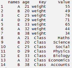
- gather () – ‘ gathers’ multiple columns. Later, turns them into key pairs: value. This function will transform from broad form of data to long form. You can use it as an alternative to 'melt’ in the remodel package.
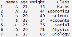
- spread (): it is reversed to collect. Take a key pair: value and converts it to separate columns.
- break apart (): split a column into multiple columns.
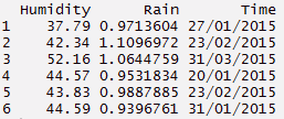
- unite (): is reversed or separated. Join multiple columns into a single column
Let's understand closely using the following code:
#load package
> library(tidyr)
#create a dummy data set
> names <- c('A','B','C','D','E','A','B')
> weight <- c(55,49,76,71,65,44,34)
> age <- c(21,20,25,29,33,32,38)
> Class <- c('Maths','Science','Social','Physics','Biology','Economics','Accounts')
#create data frame > tdata <- data.frame(names, age, weight, Class) > tdata#using gather function > long_t <- tdata%>% gather(Key, Value, weight:Class) > long_t
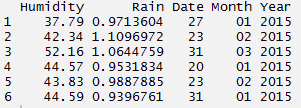
The separate function is best used when we are provided with a datetime variable in the dataset. Since the column contains multiple information, it makes sense to split it up and use those values individually. Using the code below, I have separated a column in date, month and year.
#create a data set
> Humidity <- c(37.79, 42.34, 52.16, 44.57, 43.83, 44.59)
> Rain <- c(0.971360441, 1.10969716, 1.064475853, 0.953183435, 0.98878849, 0.939676146)
> Time <- c("27/01/2015 15:44","23/02/2015 23:24", "31/03/2015 19:15", "20/01/2015 20:52", "23/02/2015 07:46", "31/01/2015 01:55")
#build a data frame
> d_set <- data.frame(Humidity, Rain, Time)
#using separate function we can separate date, month, year
> separate_d <- d_set %>% separate(Time, c('Date', 'Month','Year'))
> separate_d
 #using unite function - reverse of separate
> unite_d <- separate_d%>% unite(Time, c(Date, Month, Year), sep = "/")
> unite_d
#using unite function - reverse of separate
> unite_d <- separate_d%>% unite(Time, c(Date, Month, Year), sep = "/")
> unite_d
 #using the spread function - reverse compilation> wide_t % spread (key, value)> wide_t
Lubridate Package
The Lubridate package reduces the hassle of working with the data time variable in R. The built-in function of this package offers a good way to facilitate the analysis of dates and times. This package is frequently used with data comprising point data. Here I have covered three basic tasks performed with Lubridate.
This includes update function, duration function and date extraction. As a beginner, know these 3 functions will give you enough experience to deal with time variables. Even if, R has built-in functions to handle dates, but this is much faster. Let's understand using the following code:
> install.packages('lubridate')
> library(lubridate)
#current date and time
> now()
[1] "2015-12-11 13:23:48 IS"
#assigning current date and time to variable n_time
> n_time <- now()
#using update function
> n_update <- update(n_time, year = 2013, month = 10)
> n_update
[1] "2013-10-11 13:24:28 IS"
#add days, months, year, seconds
> d_time <- now()
> d_time + days(1)
[1] "2015-12-12 13:24:54 IS"
> d_time + dweeks(2)
[1] "2015-12-12 13:24:54 IS"

> d_time + dyears(3)
[1] "2018-12-10 13:24:54 IS"

> d_time + dhours(2)
[1] "2015-12-11 15:24:54 IS"

> d_time + dminutes(50)
[1] "2015-12-11 14:14:54 IS"

> d_time + dseconds(60)
[1] "2015-12-11 13:25:54 IS"
#extract date,time
> n_time$hour <- hour(now())
> n_time$minute <- minute(now())
> n_time$second <- second(now())
> n_time$month <- month(now())
> n_time$year <- year(now())
#check the extracted dates in separate columns
> new_data <- data.frame(n_time$hour, n_time$minute, n_time$second, n_time$month, n_time$year)
> new_data

Note: The best use of these packages is not in isolation but together. You can easily use this package with dplyr, where you can easily select a data variable and extract the useful data from it using string command.
Final notes
These packages would not only enhance your data manipulation experience, they would also give you reasons to explore R in depth. Now that we have seen, these packages make it easy to encode in R. No need to write long codes anymore. Instead, write shortcodes and do more.
Each package has multitasking capabilities. Therefore, I suggest you get an important function that can be used frequently. Y, once you get acquainted with them, you can go deeper. I initially made this mistake. I tried exploring all the functions of ggplot2 and ended up in confusion. I suggest you practice these codes while reading. This would help you build confidence in using these packages..
In this article, I have explained the use of packages 7 R that can make data exploration easier and faster. R known for its incredible statistical functions, with recently updated packages, also makes it a favorite tool of data scientists.





